Reducing Human Annotation Costs with Active Learning Techniques
Active learning selects the most informative unlabeled samples for human annotation. This tutorial covers uncertainty sampling, diversity-based sampling, and qu
Active learning aims to select the unlabeled samples that are most informative and ask for labels only for those samples. By interactively querying a user (or some other information source) to label new data points, we can train models using fewer labels. This tutorial walks you through the active learning workflow and shows you how to implement three commonly used query strategies: uncertainty sampling, diversity-based sampling, and query by committee. We provide intuitive explanations of these methods along with Python implementations. Finally, we discuss the pros and cons of each method and how they can be used together to create powerful human-in-the-loop systems when annotation is expensive or scarce.
Table of Contents
1. What Is Active Learning
Active learning is an approach to machine learning in which a learning algorithm is able to interactively query a user (or some other information source) to obtain the desired outputs at new data points. In active learning, rather than feeding a learning algorithm a massive pool of labeled examples, you allow the model to look at the unlabeled data points first. It will pick the data points it wants to learn from and send only those to the human for labeling. You repeat this process in cycles. Using active learning, you can often achieve comparable performance to normal supervised learning with many fewer annotated training examples. See Figure 1 for the active learning cycle.

Figure 1. Diagram of the active learning iterative process (source: doi.org/10.1109/ACCESS.2025.3624650)
Particularly when humans are in the loop, this technique shines. Rather than having the annotator label thousands of simple or redundant samples, the model instead surfaces which examples it is least certain about or which examples appear to be outliers, and then has the annotator label those.
To understand the significance of active learning, consider an image classification task with 500,000 images. At 20 seconds per image, it would take over 2,700 hours to label the entire dataset. With active learning, you only request human attention for the images that actually need it to improve your model substantially, drastically cutting costs and labeling effort.
1.1. Learning From Uncertain or Edge-Case Samples
One major benefit of active learning is that your model can focus on learning from the most difficult examples. These examples typically fall around the decision boundary where the model is most uncertain and have the largest potential to improve performance.
This effectively enriches your dataset with targeted samples. The dataset size does not grow through synthetic transformations, but it gains valuable information with the addition of carefully selected new samples.
Imagine training a model for self-driving cars. There are rare events that may not appear frequently enough in raw collected data — a cyclist emerging from behind a parked car is a good example. With active learning, these rare cases can be surfaced early and delivered to human annotators for review. The same applies to a fraud detection model, where you may want the model to direct human reviewers toward suspicious activity rather than transactions that are clearly legitimate or clearly fraudulent.
You can run and download the companion notebook here: https://github.com/lucasbraga461/active-learning/blob/main/active-learning/notebook.ipynb
The research paper behind this implementation is available as free access here: https://doi.org/10.1109/ACCESS.2025.3624650
2. Active Learning Techniques
The intuition behind active learning is using a query strategy to determine which unlabeled samples should be labeled first. Rather than randomly picking samples from our pool, we query the model about which samples it would like to examine — typically those that will help the model make better predictions. Active learning tends to be most useful when labels are slow to acquire, require expert knowledge, or are costly.
There are many strategies that generally trade off exploration and exploitation of the regions where the model has the largest uncertainties. These methods have been applied in vision-based tasks, document classification, anomaly detection, and medicine.
Below we cover three of the most common query strategies: uncertainty sampling, diversity-based sampling, and query by committee.
Dataset note: The examples in this article use a synthetic dataset created for demonstration purposes only.
2.1. Uncertainty Sampling
Uncertainty sampling is often the first approach practitioners attempt because it requires very little effort and often leads to good initial gains.
The concept is straightforward. You start by labeling only enough samples to create an initial training set, then train your initial model on those samples. This initial model does not have to be great — all it needs to do is make rough probability estimates for the unlabeled samples. Once trained, you identify the samples about which the model is least certain, typically those for which it predicts probabilities close to the decision threshold. You then have those uncertain samples labeled by a human and retrain the model on the expanded dataset.
Repeating this process allows the model to incrementally improve its understanding in the regions where it is least confident, producing faster gains than labeling many easy or redundant examples would.
2.1.1. Train the First Model With Cross-Validation
Before querying uncertain samples, we first need a model that performs reasonably well even when little labeled data is available. A straightforward way to accomplish this is to split the labeled data into training and validation folds, then run a small hyperparameter search using cross-validation to prevent overfitting. The result of splitting the dataset in Code Block 1 can be seen in Figure 2.
Code Block 1. Split X and y
X = df_i1.drop(columns=['label'])
y = df_i1['label']
X
Figure 2. Visualization of the dataframe independent features (X)
Teams usually run lighter grid searches with 3 or 5 folds in practice, so you do not need many folds when applying this process to your own projects.
Code Block 2. Train a model using nested cross-validation.
# Hyperparameter grid and CV settings
param_grid = {"C": [0.001, 0.01, 0.1, 1, 10, 100]}
inner_cv = StratifiedKFold(n_splits=5, shuffle=True, random_state=42)
outer_cv = StratifiedKFold(n_splits=5, shuffle=True, random_state=7)

fold_metrics = []
best_params_each_fold = []

for train_idx, test_idx in outer_cv.split(X, y):
    X_train, X_test = X.iloc[train_idx], X.iloc[test_idx]
    y_train, y_test = y.iloc[train_idx], y.iloc[test_idx]

    grid = GridSearchCV(
        LogisticRegression(max_iter=500),
        param_grid,
        cv=inner_cv,
        scoring="f1",
        n_jobs=-1
    )
    grid.fit(X_train, y_train)

    best_model = grid.best_estimator_
    best_params_each_fold.append(grid.best_params_)

    preds = best_model.predict(X_test)
    fold_metrics.append({
        "precision": precision_score(y_test, preds),
        "recall": recall_score(y_test, preds),
        "f1": f1_score(y_test, preds)
    })

# Use the most frequent best parameters to train the final model
final_params = pd.DataFrame(best_params_each_fold).mode().iloc[0].to_dict()
final_model = LogisticRegression(**final_params, max_iter=500)
final_model.fit(X, y)
Now that we have our cross-validated model, we can apply it to the unlabeled set to get a measure of uncertainty. Figure 3 shows what fold_metrics looks like from Code Block 2.

Figure 3. Cross-validation results and best parameters
2.1.2. Score the Unlabeled Data and Inspect the Probabilities
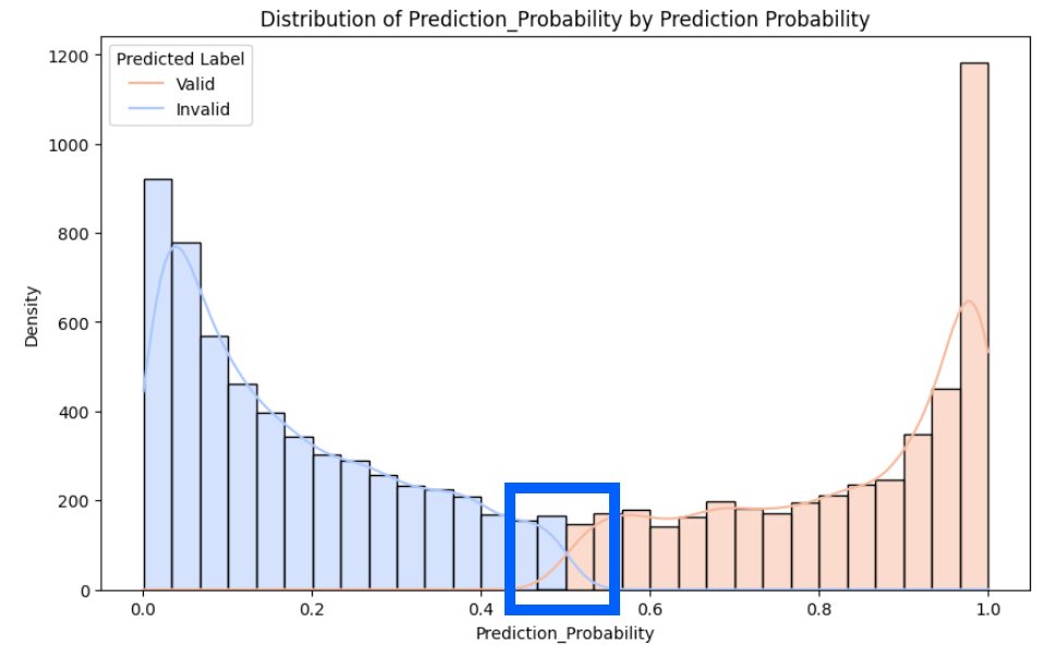
We now want to calculate predicted probabilities for every sample in our unlabeled pool. Plotting these scores helps us see where the model is least confident.
Code Block 3. Visualize the distribution of the predicted scores
import seaborn as sns

def plot_prediction_distribution(df, column_name):
    if column_name not in df.columns:
        raise ValueError(f"Column '{column_name}' not found in dataframe.")

    if "Prediction_Probability" not in df.columns:
        raise ValueError("Column 'Prediction_Probability' not found in dataframe. Ensure predictions were added.")

    plt.figure(figsize=(10, 6))
    sns.histplot(df, x=column_name, hue="Predicted_Label", bins=30, kde=True, palette="coolwarm")

    plt.title(f"Distribution of {column_name} by Prediction Probability")
    plt.xlabel(column_name)
    plt.ylabel("Density")

    plt.legend(title="Predicted Label", labels=["Valid", "Invalid"])
    plt.show()

from helpers import prediction_plots

# Get probability scores
new_probabilities = final_model.predict_proba(X_unlabeled)[:, 1]
X_unlabeled["Prediction_Probability"] = new_probabilities
prediction_plots.plot_prediction_distribution(X_unlabeled, "Prediction_Probability")
Because this is a binary classification problem, the model will often be least certain for samples with probabilities near 0.5. This region represents where active learning can be most valuable, and Figure 4 shows the resulting distribution plot from Code Block 3.

Figure 4. Distribution of prediction probabilities by predicted label
By focusing annotation effort on the samples clustered near the 0.5 threshold, each new label carries the maximum potential to shift the decision boundary and improve model performance — making uncertainty sampling a highly efficient starting point for any active learning pipeline.