Difference-in-Differences vs. Lagged Outcome Regression Explained
A simulation study comparing two causal inference methods, showing when each assumption fails and how to choose between them.
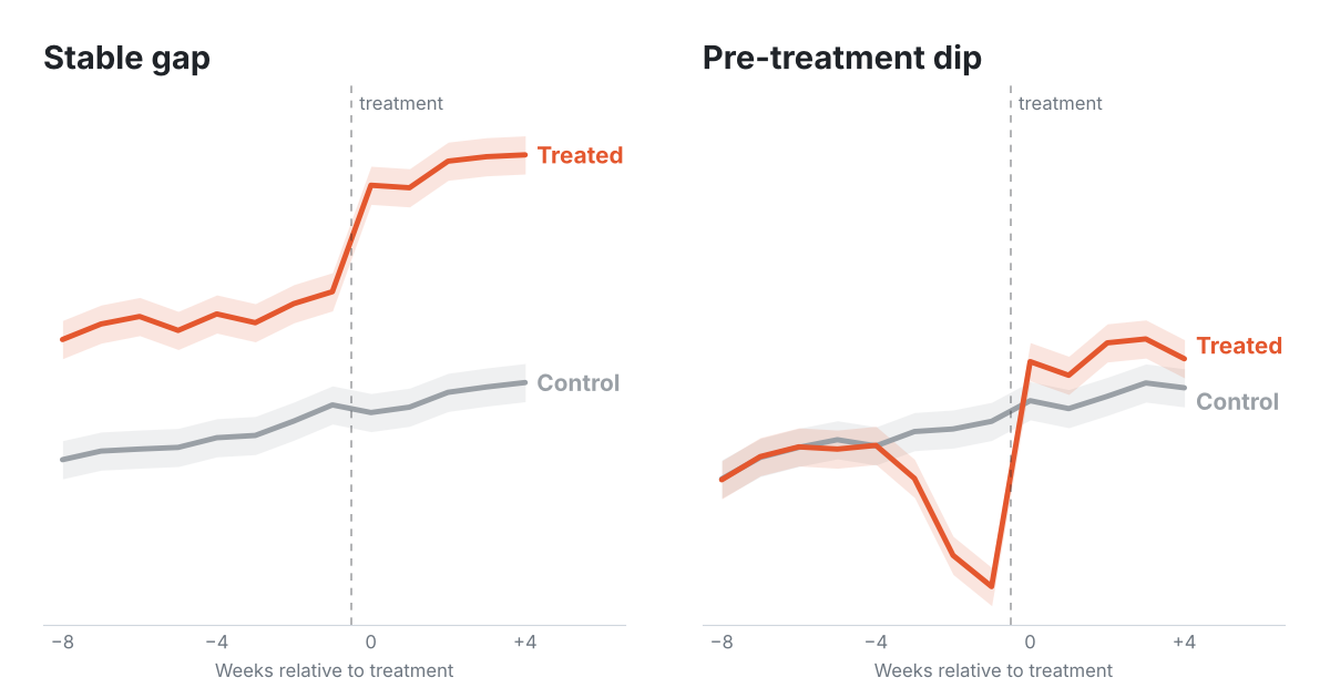
Most treatments in product analytics are chosen by the user. Someone turns on a feature, joins a community, or starts a free trial of a premium tier. There is no randomisation, but under the right assumptions we can still estimate the effect of these self-selected treatments. Without a valid instrument or a cut-off to exploit (the settings for instrumental variables or regression discontinuity), analysts tend to fall into one of two camps:
- Lagged-outcome regression, usually estimated with double machine learning. This camp learned from Causal Inference for the Brave and True and uses libraries like EconML and CausalML.
- Difference-in-differences, learned from The Mixtape and brought up to date by papers like Sant’Anna and Zhao’s Doubly Robust Difference-in-Differences Estimators (2020).
Both are reasonable, and both can be estimated with the same doubly robust machinery (DoubleML, for example, implements both). That is the point this article is built around: the estimator and the identifying assumption are separate choices, and the assumption decides whether the answer is right.
- Lagged-outcome regression assumes unconfoundedness: no unobserved confounding once you condition on past outcomes and covariates.
- Difference-in-differences assumes parallel trends: without treatment, treated and control outcomes would have moved together.
This simulation study shows when each assumption fails and gives a rule for choosing between them.
1. Lagged Outcomes and Difference-in-Differences
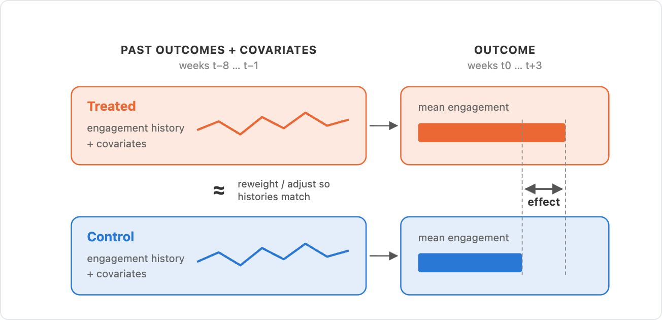
Lagged-outcome regression compares treated and control users who had the same engagement history and characteristics before treatment. After re-weighting or adjusting so those histories match, the difference in post-period engagement is the effect.
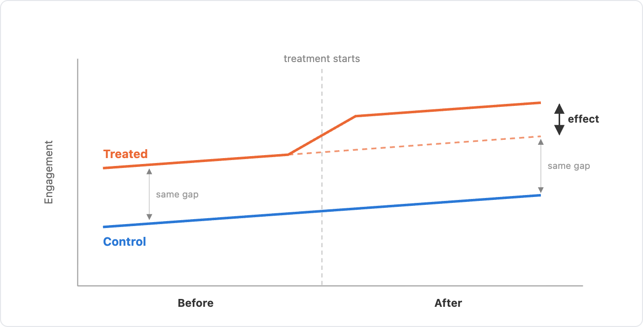
Difference-in-differences lets the two groups start at different levels. It assumes the gap between them would have stayed the same without treatment, so any change in the gap after treatment is the effect. In practice DiD is usually conditional: parallel trends only need to hold among users with the same characteristics, measured before the pre-period.
Lagged-outcome regression can be estimated by regression adjustment, inverse propensity weighting, or double machine learning. Difference-in-differences has the same menu, from two-way fixed effects to doubly robust DiD.
Doubly robust means the estimate survives a wrong outcome model or a wrong propensity model. It does nothing if the identifying assumption fails.
A useful way to see the difference is to write the post-period outcome as a function of the pre-period outcome:
$$Y_{\text{post}} = \alpha + \tau D + \beta, Y_{\text{pre}} + \gamma^{\prime} X + \varepsilon$$
Here D is the treatment, τ the effect, and X the observed covariates. τ is the treated–control gap after adjusting for Y_pre and X.
- Difference-in-differences sets β = 1. Subtract Y_pre from both sides and τ becomes the treated–control difference in each user’s change. This treats every pre-period gap as permanent: whatever separated the groups before treatment carries into the post-period in full.
- Lagged-outcome regression estimates β. Pre-period engagement mixes a lasting level with temporary shocks that fade, such as a busy week or a holiday, so the estimate lands below 1. This treats part of every pre-period gap as temporary: a group that started low is expected to recover partly on its own.
Each design is biased when the gap between the groups is not the kind it assumes. That happens in two common situations.
2. Two Failure Modes
Failure Mode 1: A Time-Invariant Confounder
Take a free trial of a premium tier. Higher-income users are more likely to start it, and they also tend to engage more every week. Income rarely changes over a few months and is usually not in your data. That makes it an unobserved, time-invariant confounder.
DiD handles this: a constant difference between users cancels when you subtract the pre-period. Lagged-outcome regression can only adjust for income as far as past engagement reveals it, so part of the difference ends up in the estimate.
Failure Mode 2: Selection on a Temporary Dip
Users often opt in when something has just changed. Take a win-back campaign: users whose activity has slipped are offered a free trial of a premium tier, and the ones who accept are disproportionately in a temporary slump. Many of them would have bounced back anyway. Ashenfelter (1978) found the same pattern in job training: trainees’ earnings fall just before they enrol and recover afterwards, whether the training worked or not.
DiD subtracts each user’s pre-period, and its covariates are measured before it, so nothing in the design accounts for the dip. The pre-period is depressed, and the recovery is counted as part of the effect. A dip that hits treated and control users alike, such as a holiday week, is not a problem, because the control change absorbs it. Lagged-outcome regression conditions on the dip itself: it compares dipped treated users with controls who dipped the same way.
To measure these biases we need data where the true effect is known, so the next section simulates it.
3. A Simulation with a Known Answer
The simulation builds a weekly panel of 10,000 users. Each user’s weekly engagement (think minutes per week, around 30 for a typical user) is the sum of four parts:
- a level set by observed covariates and an unobserved time-invariant confounder
- a trend that depends on the observed covariates
- seasonality shared by everyone
- a temporary shock that fades by 20% a week
Every user gets a candidate week. Treated users opt in that week, and controls are users who were eligible that week and did not. The feature adds 2 minutes a week for every treated user, so the true effect is 2.0. Engagement with and without the feature is simulated for every user, which is what lets us plot the true counterfactual below.
What changes between scenarios is why users opt in. In every scenario, users with lower engagement are more likely to opt in.
The four selection scenarios
| Scenario | Users opt in based on | Unconfoundedness | Parallel trends |
|---|---|---|---|
| a. Observables only | observed covariates | holds | holds |
| b. Time-invariant confounder | covariates and the time-invariant confounder | fails | holds |
| c. Temporary dip | covariates and engagement over the last three weeks | holds | fails |
| d. Both | all of the above | fails | fails |
The raw data shows each mechanism: in scenario a, the groups differ only through observed covariates; in b, treated users sit lower every week but move in parallel; in c, treated users dip in the three weeks before opting in; and d has both.
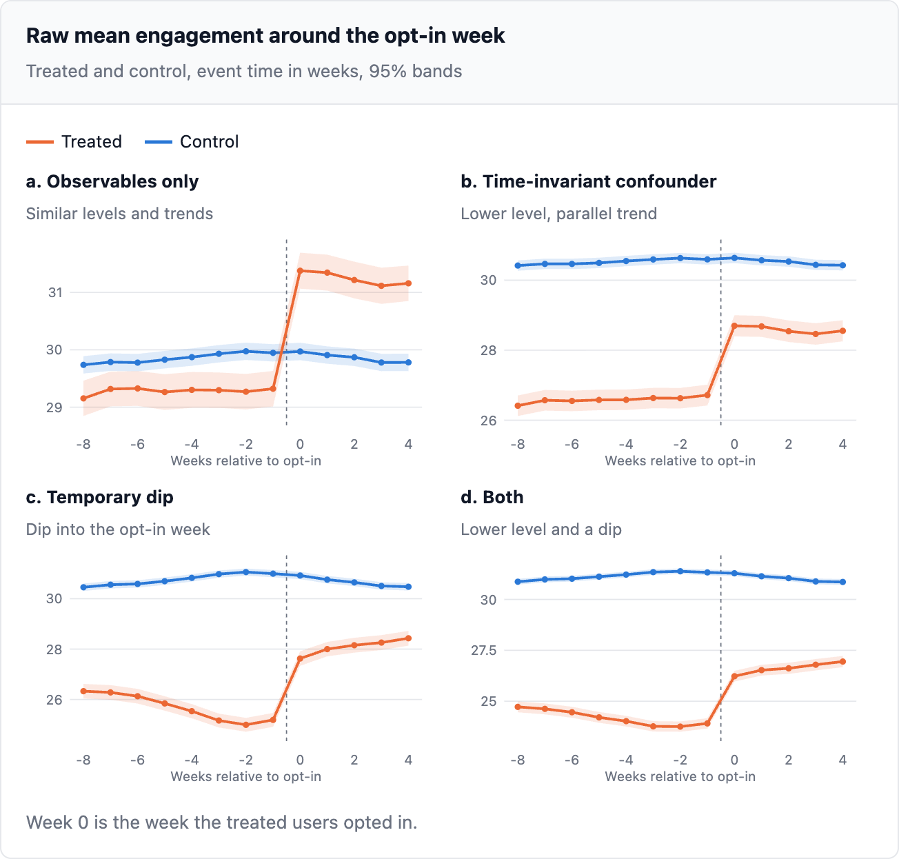
On each dataset both designs are estimated the same way, with double machine learning in DoubleML. Lagged-outcome regression uses DoubleMLIRM with the ATTE score on mean engagement in weeks 0 to 3. DiD uses DoubleMLDIDBinary on the mean over the baseline window (weeks -4 to -1) and the post-period mean (weeks 0 to 3). Both use LightGBM for the outcome and propensity models, five-fold cross-fitting, and propensities clipped at 0.01.
The next chart shows the treated users only. Orange is what they did, black dashed is what they would have done without the feature, and each coloured line is what a design assumes they would have done. A design’s estimate is the gap between orange and its own line after week 0.
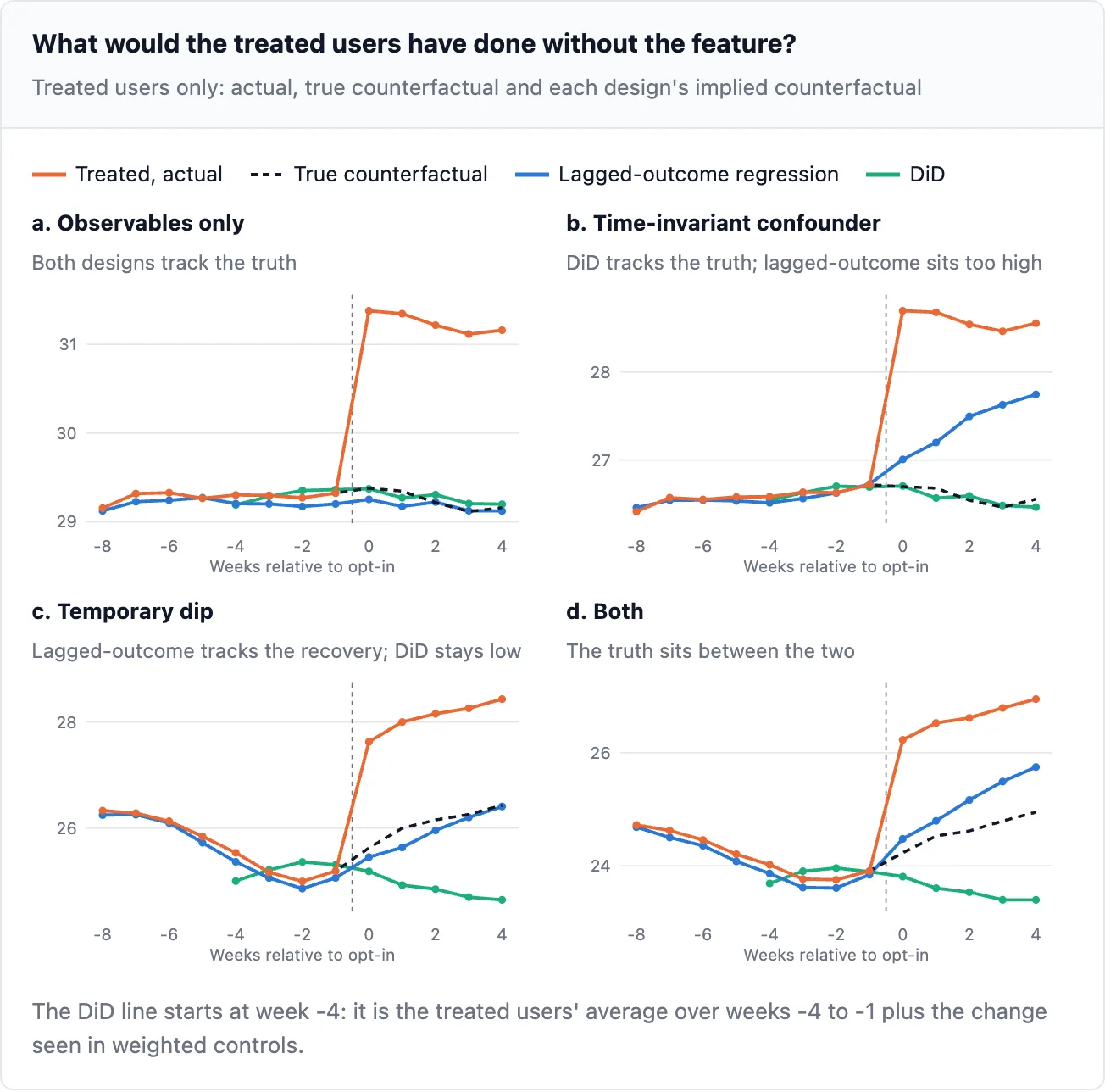
- a. Both lines sit on the true counterfactual. Both estimates are right.
- b. DiD tracks the truth. The lagged-outcome line rises after week 0 because its matched controls drift back up (failure mode 1), so it understates the effect.
- c. The true counterfactual climbs back as the dip wears off. Lagged-outcome regression follows it. DiD stays at the dipped baseline (failure mode 2), so it overstates the effect.
- d. The lagged-outcome line sits above the truth and the DiD line below it. One estimate is too small and the other too large, so the truth sits between them.
One dataset shows one draw. To see the typical estimate and its spread, each scenario was simulated 200 times and both designs were estimated on every replication.
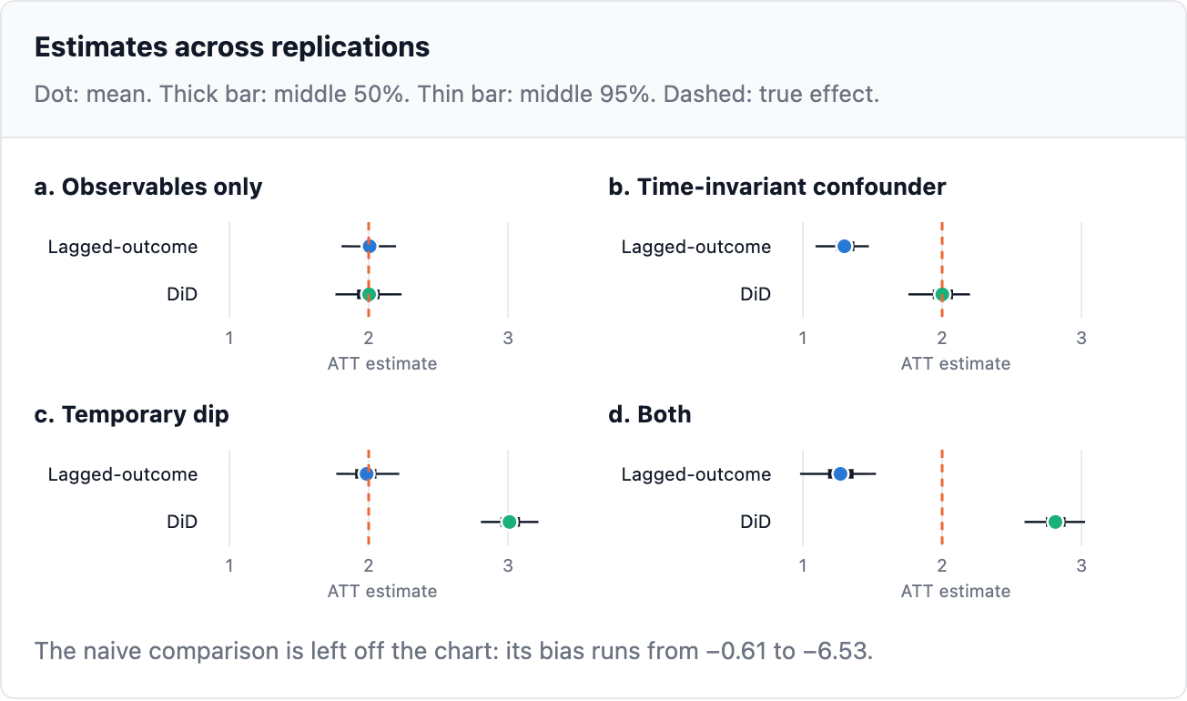
Each design is unbiased where its assumption holds and badly biased where it does not. The biased designs also produced narrow confidence intervals, meaning they fail quietly — in scenario b, DiD’s 95% intervals contained the true effect in 94% of replications, while the lagged-outcome estimator’s intervals missed it in the same proportion. This underscores the core message: choosing the right identifying assumption matters far more than the choice of estimator, and a well-implemented doubly robust method cannot compensate for a violated assumption.