Separating Shot Selection from Shot Making Using Python

Introduction

Imagine two NBA players who both shoot 40% from the three-point range.

One takes mostly open catch-and-shoot attempts from the corners. The other regularly attempts difficult pull-up threes, often with a defender in front of him.

Looking at their shooting percentages alone, we might conclude that they are equally good shooters.

But are they?

In sports, we tend to oversimplify things that aren’t simple. Field-goal percentage, for example, reflects both the difficulty of the shots a player takes and their ability to make them. And this makes player evaluation more complicated than it initially seems.

What if we could estimate the probability of making every shot based on its characteristics, and then compare that probability with the actual outcome?

That would give us two useful pieces of information:

• Shot selection: How valuable are the shots a player takes, on average?
• Shot making: How many points does the player score above or below what we would expect from those shots?

In this article, we’ll build a simple expected field-goal model using Python. We’ll use it to illustrate how these two components can be separated, and discuss what this approach can and cannot tell us about shooting ability.

One important note: because we don’t care about the players themselves and don’t want to turn this into a post trying to determine if player A is better at shooting than player B, we’ll use randomized synthetic data. If you wish to run it on any particular set of players with real-world data, you can do so as well. The complete code is available in the GitHub repository.

1. Why Field-Goal Percentage Is Not Enough

Consider the following hypothetical players:

Player	2P%	3P%	Three-point attempts
Player A	62%	38%	500
Player B	48%	38%	500

Can you tell which one is the better shooter? It’s impossible to say without more data. Player A might take many shots close to the basket, while Player B attempts more difficult two-point jumpers.

Even three-point percentage has limitations. A catch-and-shoot attempt from the corner is not equivalent to a heavily contested pull-up three from well beyond the arc.

Shot difficulty depends on much more than location. Defender distance, the type of shot, time remaining on the shot clock, and the player’s movement can all matter.

We’ll start with a simpler model, using features that can be represented in almost any basic shot-level dataset:

• Shot distance
• Whether the attempt is a two-pointer or a three-pointer
• Shot type, such as a layup, jump shot, or floater
• Whether the three-pointer comes from the corner
• Whether the shot occurs late in the shot clock

This is a deliberately simple model, so we accept not capturing every aspect of shot difficulty.

2. The Data

We’ll be using shot-chart data, similar to the NBA’s. For each shot, we need a set of features and a binary outcome indicating whether the attempt was a basket or not.

The dataset used in this walkthrough has 12 players (Player A to Player L), limited to 18,000 shots — 1,500 per player — with varied characteristics: some near the basket, some jump shots, some three-pointers. Here’s a sample:

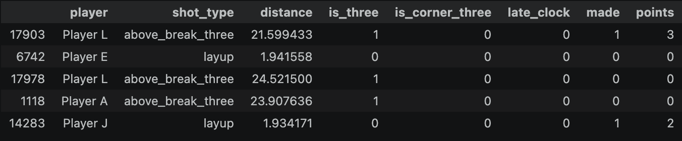
The columns are: player, shot_type, distance, is_three, is_corner_three, late_clock, made, points.

As for shot type, only four possible values are used:

• mid-range
• corner-three
• layup
• above_break_three

3. Building an Expected Field-Goal Model (xFG%)

A natural starting point is logistic regression.

Since our target variable is binary (a shot is either made or missed), logistic regression is a great fit. It estimates the probability of a successful attempt given its features.

For shot i, we can express this as:

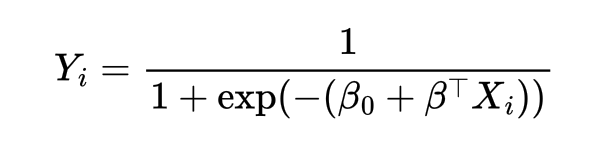
Here, Y_i is the shot outcome, X_i represents the shot characteristics we defined, and the coefficients are learned from the data.

The resulting prediction is our expected field-goal percentage for that attempt, or xFG%.

Fitting the model is straightforward using scikit-learn. After splitting the dataset and applying minimal preprocessing, we evaluate results using three metrics:

• Log loss penalizes incorrect probability estimates, particularly confident ones.
• ROC AUC measures how well the model ranks made shots above missed shots.
• Brier score measures the mean squared difference between predicted probabilities and binary outcomes.

None of these metrics alone guarantees that the predicted probabilities are well calibrated. We should also compare predicted and observed shooting percentages across groups of shots with similar predicted probabilities.

4. From Expected Shooting Percentage to Expected Points

We now have an estimated probability that each shot will go in. But there is a small problem with comparing players using xFG% alone: a made three-pointer is worth more than a made two-pointer.

A better approach is to compute the expected points per shot (xPPS) using the already-built xFG% model:

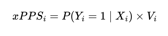
where V_i is the value of the attempt — either two or three points.

The difference between actual points and expected points gives us a shot-level measure of overperformance or underperformance.

As an example: a shot with an xFG% of 40% contributes 1.2 expected points if it is a three-pointer, but only 0.8 expected points if it is a two-pointer. This distinction matters.

5. Separating Shot Selection from Shot Making

This is where things get interesting. We now aggregate results by player and, for each one, calculate:

• Field-goal percentage
• Expected field-goal percentage
• Expected points per shot
• Actual points per shot
• Points above expectation per 100 attempts

That last measure is particularly useful. It tells us how much a player overperforms or underperforms the expected value of their attempts, expressed on a comparable scale.

Here’s what the player summary looks like:

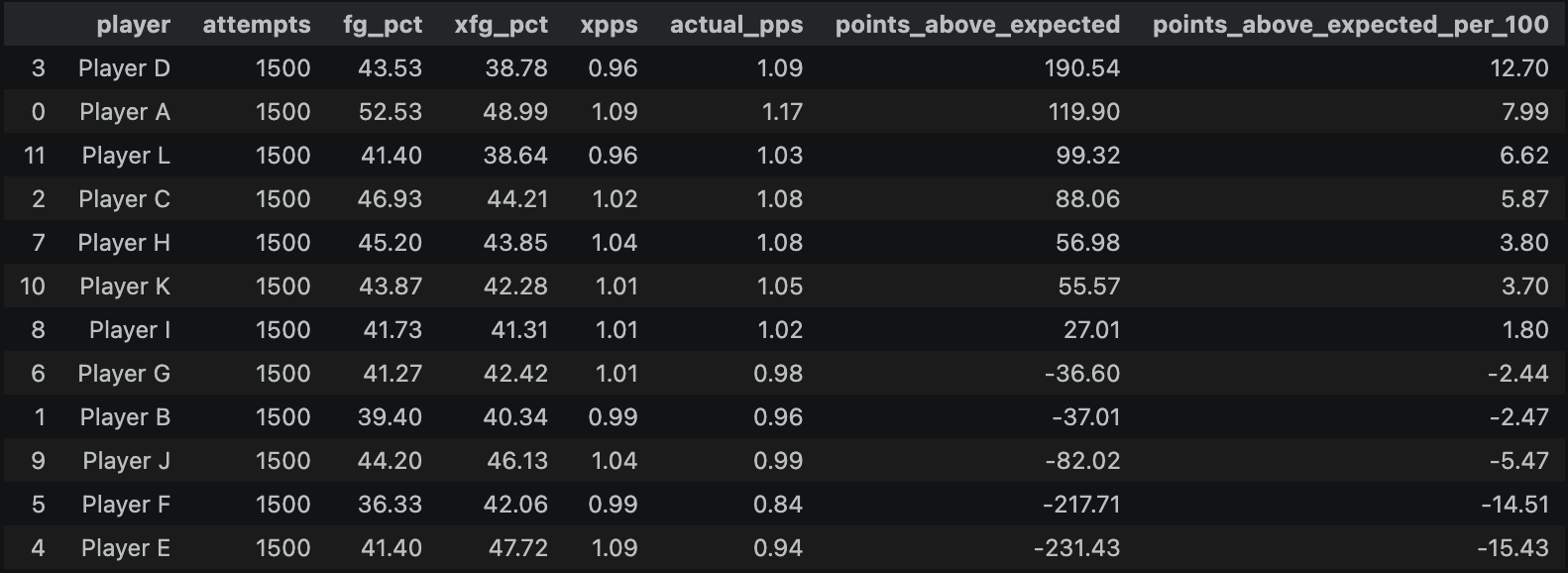
This gives us two different perspectives on a player’s shooting performance:

• Shot selection is represented by the average expected points per attempt. Players who consistently generate valuable attempts will tend to have a higher xPPS.
• Shot making is represented by the difference between actual and expected points. A positive value means the player converted their attempts into more points than the model expected.

These two measures answer different questions, and neither should be interpreted as a complete measure of shooting talent.

For example, a player could have a high expected points per shot but consistently underperform that expectation. Another player might take more difficult shots, resulting in lower expected points per shot, while regularly exceeding those expectations.

The distinction is useful because it helps us avoid treating all differences in shooting efficiency as differences in shooting ability.

6. Visualizing the Results

A table is useful for inspecting individual players, but visualizations make it easier to see how two different measures relate. Two figures are enough to study them.

The first is a shot-selection vs. shot-making chart:

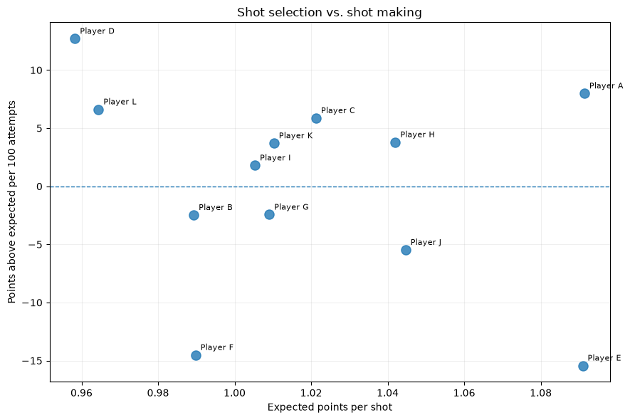
Since we’re using the normalized per-100 metric, it’s fair to compare all players. The horizontal axis measures the expected value of a player’s shot diet and the vertical axis measures the difference between actual and expected scoring.

This gives us four broad interpretations:

• High xPPS, positive residual: valuable attempts and above-expected conversion.
• High xPPS, negative residual: valuable attempts but below-expected conversion.
• Low xPPS, positive residual: less valuable attempts, but above-expected conversion.
• Low xPPS, negative residual: less valuable attempts and below-expected conversion.

The second chart compares FG% against xFG%:

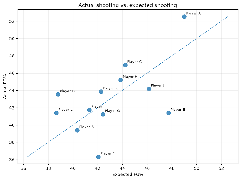
Each dot represents a player, showing whether their actual field-goal percentage lands above or below the model’s expectation. Together, these two visualizations give a clearer picture of where a player’s shooting value actually comes from — the quality of shots they select, the ability to convert them, or both.