Feature Election: Federated Feature Selection Without Sharing Data

The Suggested Preprocessing Step

Picture three hospitals that want to train one model together. Their tables share a schema, so every site has the same columns, but each holds different patients and none may send its rows to anyone else. This is horizontal federated learning: the features are shared, the rows are split across sites, and the model is trained where the data lives. The standard recipe is FedAvg (McMahan et al., 2017), in which each site trains locally, sends its weights to a server, and the server averages them, weighted by each site’s sample count.

On a pooled table, feature selection is routine. You would fit a Lasso, check random forest importances, or call SelectKBest and drop unnecessary columns. In federated learning there is no pooled table to run those tools on, and FedAvg never asks which features belong in the model. It averages whatever weights it receives, so every irrelevant feature rides along in every update, every round, and adds noise that the smaller sites feel most.

This article is about Feature Election, a method developed to address that gap. Most research on federated feature selection asks you to adopt a new purpose-built algorithm. Fed-FiS (Banerjee et al., 2021) and Fed-mRMR (Hermo et al., 2024) federate mutual-information filters, the latter by having each site share a matrix of co-occurrence counts for feature values. FedSDG-FS (Li et al., 2023) learns stochastic feature gates under homomorphic encryption for vertically partitioned data, and other work searches for feature subsets with particle swarm optimization (Zhang et al., 2026). Feature Election asks for less: each site keeps the ordinary selector it already trusts, runs it on its own rows and sends a vote, and the server settles the disagreement with one tunable rule. The sections below work through the rule by hand, implement it in NumPy, run it as a real NVIDIA FLARE (Roth et al., 2022) job, report published results on model size and F1 alongside an independent benchmark, and show how to run it in Flower (Beutel et al., 2020) and NVIDIA FLARE.

The Idea Explained

Each site runs a feature selector of its choice on its local data. For every feature it produces a yes or no (together these form the mask) and a number saying how strongly it prefers that feature (the score), and it sends both to the server along with its sample count. Features that every site selected are kept and features that no site selected are dropped, whatever their scores. The contested ones go to a vote weighted by site size, and a single parameter called the freedom degree decides how many of them get in. Every site applies the resulting global mask to its columns, and ordinary federated training such as FedAvg runs on the reduced table. No rows or gradients leave a site during the election.

How the Election Works

For a table with d features, client i sends:

• S_i, a binary mask of length d, where 1 means “my selector kept this feature”.
• M_i, a vector of d preference scores (for example absolute Lasso coefficients, random forest importances or mutual information values).
• n_i, its number of training samples.

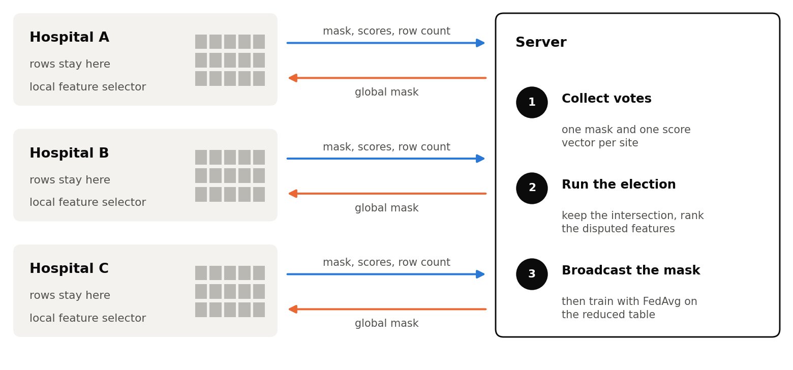
What leaves the devices during a Feature Election: masks, scores and row counts go up, one global mask returns. Data rows do not leave the site.

The server splits the features into three groups. The intersection holds the features every client selected, and these are always kept. Features no client selected are always dropped. The disputed set is the union of all selections minus the intersection: features that at least one site wanted and at least one rejected.

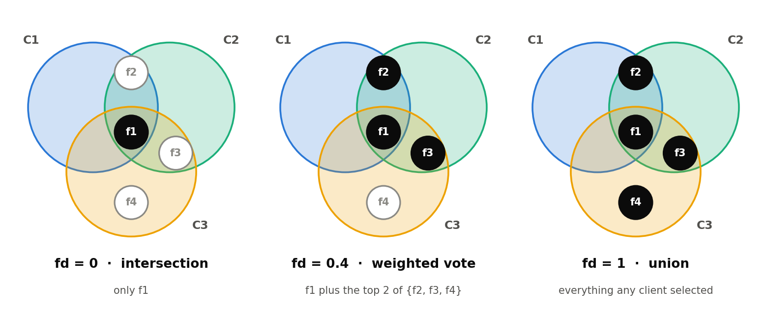
The freedom degree fd, a number in [0, 1], sets how much of the disputed set is admitted. At fd = 0 the global mask is the intersection and at fd = 1 it is the union. In between, the server min-max normalizes each client’s scores separately, so that a Lasso coefficient and a mutual information value land on the same 0 to 1 scale. It computes client weights w_i = n_i / sum(n) and an aggregated vote per feature, V = sum_i w_i * M_i, over the normalized scores. It then keeps the top ceil(fd * |disputed|) disputed features by V, on top of the intersection.

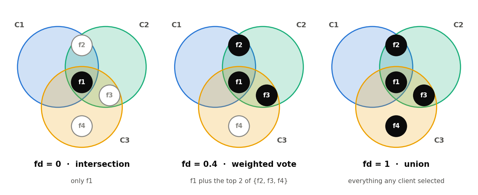
The freedom degree slides the global mask from the intersection (fd = 0) to the union (fd = 1). Filled dots are features kept in the worked example below.

The freedom degree trades off two failure modes. At fd = 0 every site holds a veto, so one site with a strict selector shrinks the model for everyone, including sites whose data needed the vetoed features. At fd = 1 every site can pollute the mask, so the noise features of one loose selector reach everyone. In between, the sites with more data and stronger preferences decide the contested cases.

A small example makes this concrete. Three clients hold 50%, 30% and 20% of the data, so their weights are 0.5, 0.3 and 0.2. Feature f1 was selected by all three. Feature f2 was selected by C1 (score 0.9) and C2 (0.6), f3 by C2 (0.8) and C3 (0.6), and f4 only by C3 (0.4). The table shows every client’s normalized score for every feature, with the scores of features that client selected in bold. A client’s score counts in the vote whether or not it selected the feature: how much C1 likes f3 can help or hurt f3 even though only C2 and C3 put it in their masks.

Feature	C1 (w = 0.5)	C2 (w = 0.3)	C3 (w = 0.2)	Vote V	Outcome at fd = 0.4
f1	selected	selected	selected	n/a (Unanimous)	kept (intersection)
f2	0.9	0.6	0.3	0.5×0.9+0.3×0.6+0.2×0.3 = 0.69	kept (rank 1)
f3	0.2	0.8	0.6	0.5×0.2+0.3×0.8+0.2×0.6 = 0.46	kept (rank 2)
f4	0.1	0.2	0.4	0.5×0.1+0.3×0.2+0.2×0.4 = 0.19	dropped (rank 3)

The disputed set is {f2, f3, f4}, and at fd = 0.4 the server admits ceil(0.4 × 3) = 2 of them, f2 and f3, giving the global mask {f1, f2, f3}. At fd = 0 the mask would be {f1} alone and at fd = 1 all four features. The weighting widens the gap: with equal site sizes f2’s vote would be 0.60 and f3’s about 0.53, so C1’s half of the data is what puts f2 clearly ahead.

The Algorithm in NumPy

The rule is short enough to write out in full. The function takes lists of masks, score vectors and sample counts and returns the global mask with a few counts. Scores go through abs so that negative Lasso coefficients vote the same way as positive ones.

Note that the masks only decide which features are in the intersection, the disputed set, or out. The vote itself uses every client’s score for a disputed feature, including clients that left it out of their mask. A feature that only the smallest site selected can still win a place if the larger sites scored it just below their own cut-off, and it will lose if they scored it near zero. This is why the function normalizes and sums the full score vectors and does not zero them with the masks.

Running It as an NVIDIA FLARE Job

The function above is for reading. For numbers, the shipped implementation runs as a FLARE job: a FeatureElectionController on the server and a FeatureElectionExecutor on each of three sites, exchanging FLARE tasks. It launches with FLARE’s simulator, which runs the server and the three clients on one machine; the same job object can be exported with job.export_job() and submitted to a provisioned federation. The module is in the nvflare package from release 2.8.0.

The table has 100 features: 12 informative, 8 redundant (linear combinations of the informative ones, so they carry signal too) and 80 noise. With shuffle=False, scikit-learn puts the 20 signal features in the first 20 columns, which makes it easy to check what the election kept. A short script, prepare_data.py, writes one CSV per site with 1,500, 900 and 600 rows. Each site needs one thing: how to load its own data. The executor reads the site’s CSV the first time a task arrives and leaves everything else to Feature Election.

The job gives every site a different selector: Lasso at the largest site, a random forest at the second, and mutual information at the smallest.

Both failure modes show up clearly in the results. On their own data the Lasso site selected 35 features with 12 of the 20 signal features among them, the random forest site selected 50 with all 20, and the mutual information site selected 50 with 15. At a freedom degree of 0 the strictest selector holds a veto, and the mask keeps only 10 signal features. At 1 every site’s noise gets in, and the mask carries 61 noise features. At 0.5 the vote recovers all 20 signal features with 28 noise features, less than half the noise of the union. Running at 0, 0.5 and 1 with two other seeds for the table confirmed the pattern: 8 and 9 signal features at 0, 19 at 0.5, and 61 and 62 noise features at 1.

Auto-tuning has one notable limitation. It tried freedom degrees between 0.5 and 0.7, saw validation F1 between 0.776 and 0.781, and settled on 0.6 with 55 features. The hill climb optimizes F1 alone, so when F1 is this flat it has no reason to prefer the smaller mask. A setting of 0.5 delivers the same signal recovery with 7 fewer noise features, which illustrates why model size should be considered alongside predictive performance when choosing the freedom degree for a given federation.