A First Look at Survival Analysis and the Cox Model

The Question Ordinary Regression Can’t Answer

Here is a dataset. 432 people were released from prison and were followed for one year. They were being watched for a single event: re-arrest. Some were re-arrested in week 8, some in week 30. Most (318 of them) reached the end of the study having never been re-arrested at all.

The simple question being asked in this study was how long until someone re-offends?

We cannot just average the arrest times. Three-quarters of the people never got arrested, so they have no arrest time to average. We cannot throw those people away either. Because if we only analyse the ones who failed, we will end up concluding that everyone eventually re-offends, which is both false and grim. And we also cannot code the survivors as arrested after week 52, because they weren’t. They were either arrested at some week after the 52nd week that we never got to see, or maybe never.

That last situation — where we know someone lasted at least this long, but we do not know how long in total — is called censoring. It is the entire reason survival analysis exists as its own field. Ordinary linear regression has no way to represent “the answer is at least 52.” It wants a number. Survival analysis is the set of tools built for the case where, for a big chunk of our data, the clock was still running when we stopped watching.

This post builds on that single problem. We will start with three core ideas needed to understand survival analysis, then move on to the following three activities:

1. Estimate a survival curve straight from data with Kaplan-Meier.
2. Spend most of our time on the Cox proportional hazards regression.
3. Fit one model in Python, reading its output as hazard ratios.

Three Core Concepts in Survival Analysis

Almost everything in survival analysis is built from three objects.

1. The event and the time: Pick one well-defined event — death, re-arrest, machine failure, subscription cancellation, or a loan default. For each subject, we record two things: how long they were observed (the duration), and whether the observation ended because the event happened or because we stopped watching (the event indicator, binary coded as 1 or 0). These two columns are the key inputs of every model below.

2. The survival function, S(t): This is the probability that a subject makes it past time t without the event. It starts at 1 at time zero and decays toward 0 over time. For example:

“Survival at 12 months is 0.7” means 70% are expected to still be event-free at a year.

3. The hazard function, h(t): The hazard is the instantaneous rate of the event at time t, given that the subject has survived up to t. Informally:

Of the people who’ve made it this far, what fraction fail right now?

The distinction between S(t) and h(t) matters. Survival is cumulative; hazard is momentary. Our overall probability of still being alive at 80 is low (survival is small), but our hazard at the exact instant we turn 80 is a different quantity entirely. Survival is how much water is left in the tank. Hazard is how fast it is draining right now. They are linked by calculus: hazard is failure density divided by survival, so integrating the hazard gives back survival.

Why obsess over the hazard rather than modelling survival directly? Because the hazard is the natural place to attach covariates. It is straightforward to say “financial aid multiplies the rate of re-arrest by 0.68 at every moment.” That sentence is a statement about the hazard, and it is exactly what the Cox model provides.

Kaplan-Meier: A Survival Curve With No Assumptions

Before modelling anything, we can estimate S(t) directly from data. The Kaplan-Meier estimator (Kaplan & Meier, 1958, one of the most-cited papers in statistics) does this without assuming any particular shape for the curve.

The idea is straightforward. Walk forward in time. At each moment where an event actually happens, look at how many people were still at risk just before and how many failed. Multiply together the “fraction who survived this instant” values as we go. Censored people contribute to the at-risk count right up until they leave, then quietly drop out without ever causing a downward step.

The specific dataset used here is the Rossi recidivism dataset, included with the lifelines Python library. It comes from a 1980 randomised experiment by Rossi, Berk, and Lenihan. The study followed 432 released prisoners for one year and recorded whether they were re-arrested, along with covariates such as race and education. Splitting the subjects into two groups — those who received financial aid after release and those who did not — produces the following curves. In the original study, this aid was assigned randomly, so the comparison is fair.

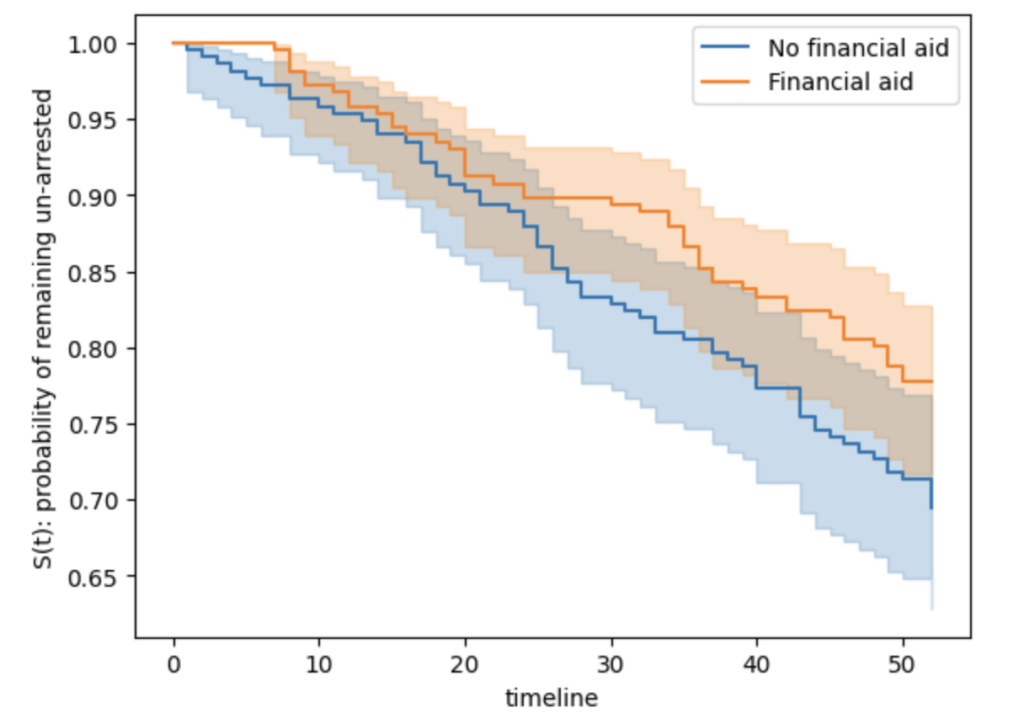
Figure 1. Kaplan-Meier curves by financial-aid group. Every downward step is a re-arrest; the shaded bands are 95% confidence intervals. The aid group (blue) stays higher throughout. By week 52, about 22% of the aid group had been re-arrested versus 31% of the no-aid group.

To test whether that gap is more than noise, the standard tool is the log-rank test. It compares the observed number of events in each group against what would be expected if the two curves were identical.

On this data, it returns p ≈ 0.05, which is right on the border. This is a good reminder that Kaplan-Meier plus log-rank is a description of one variable at a time. It cannot adjust for age, prior record, or anything else. The moment you want to control for covariates, a Cox model is needed.

The Cox Model: Regression on the Hazard

When the goal is something like regression — plug in covariates, get out their effects — but applied to the hazard, the naive move is to write down a full formula for h(t) and estimate everything. But h(t) has a shape over time, and we usually have no idea what that shape is and no desire to commit to one. Cox’s insight was that we can estimate the covariate effects without ever specifying the baseline shape. The model is:

Read it as two pieces multiplied together:

• h₀(t), the baseline hazard: the risk over time for a hypothetical subject with all covariates at zero. The shape is left completely unspecified — it can be any shape. This is the nonparametric part.
• exp(βᵀx), the covariate effect: a single number that scales the entire baseline up or down depending on personal characteristics. This is the parametric part.

Because the model is part-nonparametric and part-parametric, it is called a semiparametric model.

Here is what makes the Cox model particularly useful. Take two subjects and form the ratio of their hazards. The baseline h₀(t) is identical for both, so when the ratio is formed, the baseline appears on the top and bottom and cancels out:

The right-hand side has no t in it. The unknown, time-varying baseline is gone. The hazard ratio is therefore the same at week 1, week 20, and week 52 — and the baseline shape never needed to be specified. That cancellation is the entire magic trick.

Cox then turned this into a method called the partial likelihood. At each event time, the model asks:

Among everyone still at risk right now, how much more likely was it that this particular person failed, rather than one of the others?

Censored people fit naturally into this setup. They stay in the at-risk set until they leave the study, then quietly drop out. They never need an event. They still contribute information by indicating they were event-free up to that point.

Two things worth noting before fitting the model:

• Ties: The partial likelihood assumes events can be ordered. When two events land in the same week, software applies a correction — usually Efron’s method, which is the modern default and more accurate than Breslow’s.
• exp(β) is the hazard ratio. A coefficient of β = 0 means exp(β) = 1, i.e., no effect. β < 0 means exp(β) < 1, a protective factor that lowers the hazard. β > 0 raises it. The exponentiated version is almost always what gets reported.

Fitting the Cox Model in Python and Interpreting Hazard Ratios

The lifelines library makes fitting a Cox model straightforward. The estimated hazard ratios from the Rossi dataset are presented below:

Covariate	Hazard ratio exp(β)	95% CI	p-value
Financial aid	0.68	0.47 – 1.00	0.047
Age (per year)	0.94	0.90 – 0.99	0.009
Prior convictions (each)	1.10	1.04 – 1.16	0.001
Race	1.37	0.75 – 2.50	0.31
Work experience	0.86	0.57 – 1.31	0.48
Married	0.65	0.31 – 1.37	0.26
On parole	0.92	0.63 – 1.35	0.67

Reading the statistically significant results:

• Financial aid, HR 0.68. Receiving aid is associated with a 32% lower hazard of re-arrest at any given moment. This is the treatment effect the original experiment was built to detect.
• Age, HR 0.94. Each additional year of age lowers the hazard by about 6%. Older releasees re-offend more slowly.
• Prior convictions, HR 1.10. Each prior conviction raises the hazard by about 10%, and the effect multiplies: five prior convictions is roughly 1.10⁵ ≈ 1.6× the baseline hazard.

A hazard ratio is not a difference in survival probability. It is a multiplier on the momentary rate, assumed constant across the entire follow-up period. This raises an important follow-on question: is that constancy assumption actually satisfied?

The Assumption in the Name: Proportional Hazards

The model is called proportional hazards because the hazard ratio between any two subjects is assumed to remain constant over time. This is a strong assumption. If the effect of financial aid fades after six months, or if the protective effect of age only kicks in after a certain point, the model’s coefficients will be a distorted average rather than a reliable estimate.

Verifying this assumption is an essential step after fitting any Cox model. Standard approaches include plotting Schoenfeld residuals against time — a flat line for each covariate supports the proportionality assumption — and applying a formal statistical test. If proportionality fails for a covariate, common remedies include stratifying on that variable, adding a time-interaction term, or switching to a parametric survival model that allows the effect to vary over time.

Kaplan-Meier, the log-rank test, and the Cox proportional hazards model together form the practical core of survival analysis. Kaplan-Meier describes what happened to a single group or compares two groups without adjustment. The Cox model extends that to multiple covariates, returning interpretable hazard ratios while leaving the baseline hazard unspecified. Together they handle the fundamental challenge of censored time-to-event data in a principled and flexible way.