Encoding Categorical Data for Outlier Detection

This article is part of a series on Outlier Detection. Here we look at working with categorical data.

Generally when performing outlier detection with tabular data, we start by converting the data so that it is either entirely categorical or entirely numeric. There are some exceptions, but for the most part this is necessary: most outlier detection algorithms will assume the data is strictly in one format or the other, and we’ll need to get the data into the format the detector expects.

If the detector expects categorical data, the numeric features will need to be converted to a categorical format, which generally means binning them. And if the detector expects numeric data, any categorical features need to be numerically encoded. This is the more common scenario (the majority of outlier detection algorithms assume numeric data), and is what we’ll cover in this article.

Other articles in the series include: Deep Learning for Outlier Detection on Tabular and Image Data, Distance Metric Learning for Outlier Detection, An Introduction to Using PCA for Outlier Detection, Interpretable Outlier Detection: Frequent Patterns Outlier Factor (FPOF), and Perform Outlier Detection More Effectively Using Subsets of Features.

This article also covers some material from the book Outlier Detection in Python.

Outlier Detectors

Some examples of outlier detection algorithms that assume categorical data include: Frequent Patterns Outlier Factor (FPOF), Association Rules, and Entropy-based methods. Some that work with numeric data include: Isolation Forests, Local Outlier Factor (LOF), kth Nearest Neighbors (kNN), and Elliptic Envelope.

If you’re familiar with any outlier detection algorithms, it’s more likely the numeric algorithms, particularly Isolation Forest and LOF; these are probably the most commonly used algorithms. Further, all of the outlier detection algorithms included in scikit-learn and in PyOD (Python Outlier Detection) assume completely numeric data.

At the same time, the great majority of real-world tabular data is actually mixed (containing both numeric and categorical columns), which means it’s very common when performing outlier detection to need to encode the categorical columns.

There is a reason for this: mixed data is more difficult to perform outlier detection on. Working with data of just one type (all categorical or all numeric) does simplify the work of finding the most unusual items in the data.

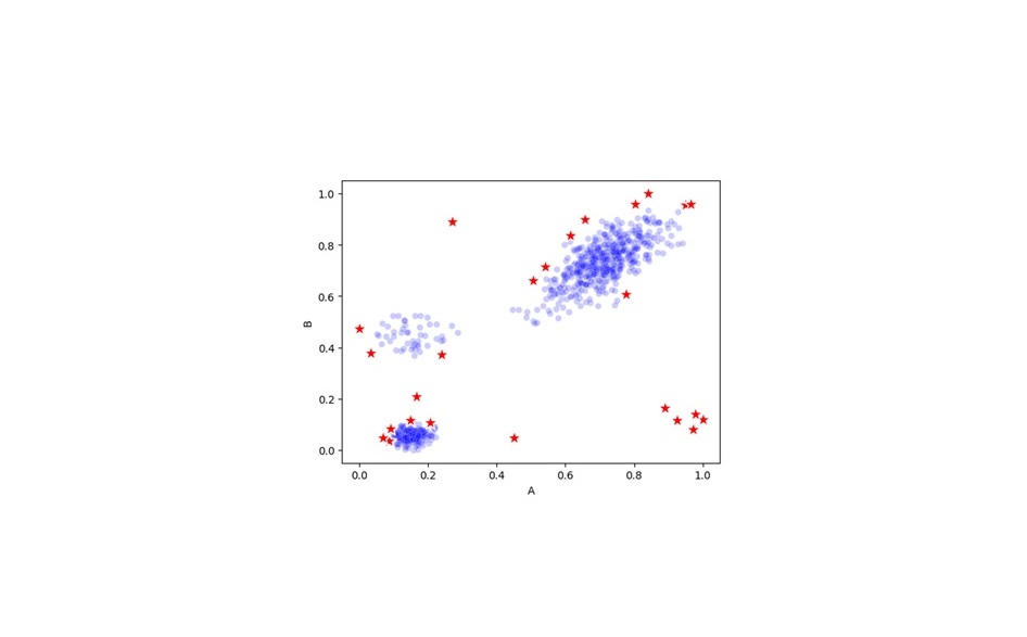
And, if we work with numeric data, we have the further benefit of being able to view the data geometrically: as points in space. If there are, say, 20 numeric columns in a table, then each row of the data can be viewed as a point in 20-dimensional space. At least, we can conceptually imagine them in 20-d space — the human mind can’t actually picture this. But we can picture 2d and 3d spaces and can extrapolate the general idea: we’re looking for points that are physically very distant from most other points. For example, in 2d, we may have data such as:

Here, we assume the data has just two features, called A and B, both with numeric values. Each row in the data is drawn either as a blue dot or a red star, with its location based on the values in the A and B columns. The blue dots indicate typical data, and the red stars represent a subset of the points that could be reasonably considered outliers: some points on the fringes of the clusters, and the points outside the clusters (the data has three main clusters, as well as some points outside these).

This is quite natural in lower dimensions. Things are different in high dimensions, due to what’s called the curse of dimensionality, and we do have to be mindful of that. But, conceptually, the idea of outliers as relatively isolated points in high-dimensional space is fairly straightforward.

Most numeric outlier detectors work by calculating the distances between each pair of points, and using these distances to identify the points that are most unusual — the points that have few points near them and that are far away from most other points. Though, in practice (for efficiency), the algorithms won’t actually calculate every pairwise distance (some can be skipped where it won’t substantially affect the outlier scores), but in principle, this is what the majority of numeric outlier detectors are doing.

We need, then, ways to convert categorical data to a numeric format that supports this well; that is, that makes it meaningful to calculate distances between rows after encoding the categorical values as numbers.

Methods to Encode Categorical Data

With prediction problems, the most common encoding methods likely include:

• One-hot encoding
• Ordinal encoding
• Target encoding

With outlier detection, the set of options is a bit different, and the strengths and weaknesses of each are also different. Out of the three methods listed here, really only one-hot encoding works well for outlier detection. With outlier detection, the most effective are likely:

• One-hot encoding
• Count encoding

This article describes how each works, and why some work better than others for outlier detection, including why count encoding (which is rarely used with prediction problems) can be quite useful with outlier detection.

Besides these encoding methods, there are several others that can be useful for prediction. An excellent library for encoding methods is Category Encoders, which will likely cover any of the methods you will need. Many of the methods provided, though, such as Target encoding and CatBoost encoding, require a target column, which is normally not available with outlier detection.

For example, if we had a table representing historical information about customers of a business, there may be a categorical column for “Last Product Purchased” and a target column called “Will Churn in next 6 Months”. The “Last Product Purchased” column may have the distinct values: “Product A”, “Product B”, and “Product C”. To encode these, we can calculate how often the target column has value True for each value (in the training data), possibly encoding these as 0.12, 0.43, 0.02 (meaning, when the “Last Product Purchased” is Product A, 12% of the time the target column is True and the client churns in the next 6 months; similarly for Product B at 43% and Product C at 2%).

But with outlier detection, we’re working in a strictly unsupervised environment: there is no ground truth value for how outlierish each row is, and so no way to set a target column. We can use only unsupervised encoding methods, including one-hot and count encoding.

One-Hot Encoding

To look at one-hot encoding, we’ll start by describing how it is done, and then examine how it works with distance calculations. Consider a table such as the following:

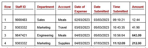
This table describes staff expenses, with one row per expense claim. Assuming we plan to use one or more numeric outlier detectors, we’ll need to convert the categorical columns (Staff ID, Department, and Account) to numbers.

The Date and Time columns will also need to be converted to numeric values. Outlier Detection in Python covers working with date and time data in detail. Briefly, they can be converted in a number of ways. One simple method is by calculating the time since some starting point (referred to as the epoch). The minimum date or time in the column may be used, or some other date that represents a logical starting point.

For example, using January 1, 1990 as the epoch, all dates can be represented as the number of days since that point. It may also be useful to capture additional information about the dates, such as the day of the week (relevant if, for example, staff expenses on weekends are unusual) or whether they fall on a holiday. For this article, though, we’ll focus just on categorical columns.

If we consider, for the moment, just the Department column, by one-hot encoding this column we replace it with a series of new columns, one for each unique value in the column. Assuming the column has five distinct values — Sales, Marketing, Engineering, HR, and Communications — we would then have five new columns representing these values, as shown in the following table.

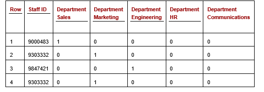
Each of the cells in the one-hot Department columns will have a value of either 0 or 1, indicating whether that is the correct value for the row. In the first row, an expense claim for Staff 9000483 who is in Sales, the column for “Department Sales” has a 1 and the other Department columns have a 0. Similarly, for each other row: exactly one of the Department columns will have a 1, and all others a 0.

One-hot encoding is very commonly used for outlier detection and can be a good choice when a feature has low cardinality. It can, though, break down somewhat where the column has very high cardinality — for example, if the Department column in the original staff expenses table had a large number of distinct values, one-hot encoding would produce a very wide, sparse set of columns that can distort distance calculations and reduce the effectiveness of numeric outlier detectors.