Classical NLP for Spooky Author Identification: From Bag-of-Words to Stacking

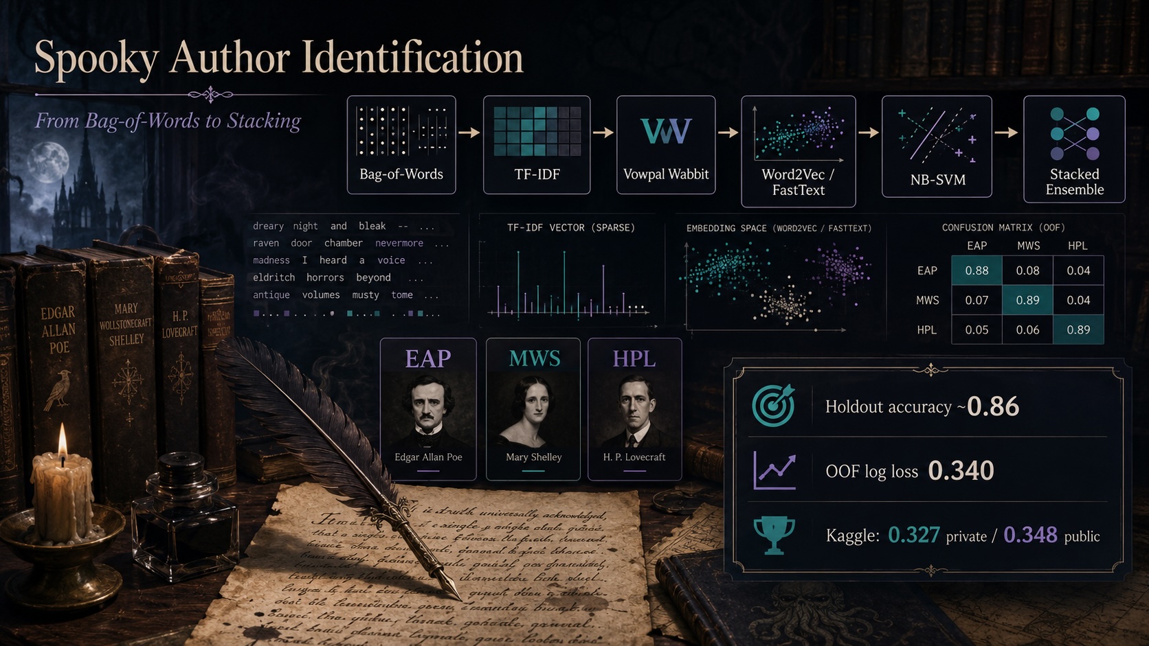
Authorship attribution is a good way to test NLP models because it focuses not only on what a sentence says, but also on how it is written. Kaggle’s Spooky Author Identification competition is a compact version of this challenge: given a single sentence from gothic or horror fiction, the model has to predict whether it was written by Edgar Allan Poe (EAP), Mary Wollstonecraft Shelley (MWS), or H. P. Lovecraft (HPL).

At first, this seems like a typical three-class text classification problem. But in reality, it is more complex. The authors all write about similar themes: fear, mystery, death, atmosphere, and the supernatural. Simple keywords are not enough to tell them apart. Instead, the important clues are often stylistic: function words, punctuation, character patterns, short phrases, sentence rhythm, and the way each author builds a sentence.

This made the project a good way to explore a specific question:

How far can classical NLP go when we choose representations carefully and evaluate them honestly?

The task was approached by building a sequence of increasingly capable classical models:

1. a fast Vowpal Wabbit word baseline,
2. a richer VW model with punctuation and character n-grams,
3. a tuned TF-IDF ensemble,
4. a stacked sparse-text ensemble using out-of-fold predictions,
5. a small representation survey comparing sparse features, BM25, Word2Vec, and FastText.

The goal was not only to improve the score, but also to understand which representations helped, which metrics improved, and which evaluation setup each result came from.

This article focuses on the project’s methodology, results, and interpretation. The main implementation choices are covered with key code snippets, but not every line from the notebook. The complete executed notebook, including the full implementation and outputs, is available in the GitHub repository linked at the end.

Dataset and Evaluation Setup

The dataset contains 19,579 labeled training sentences and 8,392 unlabeled test sentences. The class distribution is mildly imbalanced:

Figure 1. Class distribution in the training set. The dataset is mildly imbalanced, with EAP making up the largest share of examples and HPL the smallest.

Labels were encoded as 1-based integers because Vowpal Wabbit’s One-Against-All multiclass mode expects labels starting at 1.

train_texts = pd.read_csv(DATA_DIR / "train.csv", index_col="id")
test_texts = pd.read_csv(DATA_DIR / "test.csv", index_col="id")

AUTHOR_CODE = {"EAP": 1, "MWS": 2, "HPL": 3}
train_texts["author_code"] = train_texts["author"].map(AUTHOR_CODE)

print(f"Train: {len(train_texts)} sentences   Test: {len(test_texts)} sentences")
print(train_texts["author"].value_counts(normalize=True).round(3))

To compare models locally, a single stratified 70/30 train-validation split with a fixed random seed was used. This kept class proportions stable and ensured that every model was evaluated on the same held-out examples.

train_texts_part, valid_texts = train_test_split(
    train_texts,
    test_size=0.3,
    random_state=17,
    stratify=train_texts["author_code"]
)

y_part = train_texts_part["author_code"].values
y_valid = valid_texts["author_code"].values

Three main metrics were used throughout:

• Accuracy: straightforward to understand, but it only measures the final top-class decision.
• Macro-F1: useful for checking whether performance is balanced across the three authors.
• Multiclass log loss: the official Kaggle metric and the most important metric for this project, because it evaluates the quality of the predicted probabilities, not just the predicted class.

Log loss rewards confident correct predictions and heavily penalizes confident wrong predictions. This matters in a competition where the submission is a probability distribution over EAP, HPL, and MWS.

1. Word-Only Vowpal Wabbit Baseline

Vowpal Wabbit is fast, handles sparse data well, and is well-suited to linear text models. VW trains online linear models, hashes features into a fixed feature space, and handles multiclass classification through One-Against-All.

For the first baseline, only lowercased word features of length three or more were used.

def to_vw_words(df, is_train=True):
    """VW line: '<label> |text <words of 3+ chars>'."""
    lines = []

    for i in range(len(df)):
        label = df["author_code"].iloc[i] if is_train else 1
        text = df["text"].iloc[i].lower().replace("|", "").replace(":", "")
        words = " ".join(re.findall(r"\w{3,}", text))
        lines.append(f"{label} |text {words}\n")

    return lines

One implementation detail that mattered was how VW handles multiple passes. When VW reads a file directly, options such as passes and cache behave as expected. When feeding examples manually through the Python API, the file must be looped over explicitly.

N_PASSES = 10

vw = Workspace(
    oaa=3,
    loss_function="logistic",
    ngram=2,
    b=28,
    quiet=True,
    final_regressor=f"{OUTPUT_DIR}/spooky_words.vw"
)

for _ in range(N_PASSES):
    with open(f"{OUTPUT_DIR}/train_words.vw") as f:
        for line in f:
            vw.learn(line)

vw.finish()

On the 70/30 holdout split, the word-only VW baseline reached:

Holdout performance of the word-only Vowpal Wabbit baseline. Even with simple word and bigram features, the fast linear VW model provides a strong starting point.

This was already a strong result for a fast linear model using simple word and bigram features. It also established a useful baseline: any added representation or ensemble layer needed to clear this bar.

2. Rich VW: Adding Style-Aware Features

Authorship attribution involves more than classifying topics. A model also needs access to cues that reflect writing style. For the richer VW model, the input was separated into three namespaces:

• |w for words, including short function words,
• |p for punctuation,
• |c for character n-grams.

def char_ngrams(text, ns=(2, 3, 4)):
    """Boundary-aware character n-grams; whitespace/edges become '_'."""
    t = "_" + re.sub(r"\s+", "_", text.strip()) + "_"
    return [t[i:i + n] for n in ns for i in range(len(t) - n + 1)]


def to_vw_rich(df, is_train=True, char_ns=(2, 3, 4)):
    """Three namespaces: |w words, |p punctuation, |c character n-grams."""
    lines = []
    texts = df["text"].values
    labels = df["author_code"].values if is_train else None

    for i, text in enumerate(texts):
        safe = str(text).lower().replace("|", " ").replace(":", " ")

        label = labels[i] if is_train else 1
        words = " ".join(re.findall(r"\w+", safe))
        punct = " ".join(re.findall(r"[^\w\s]", safe))
        chars = " ".join(char_ngrams(safe, ns=char_ns))

        lines.append(f"{label} |w {words} |p {punct} |c {chars}\n")

    return lines

This model used more passes and a slightly larger hash space than the word-only baseline.

N_PASSES = 15

vw = Workspace(
    oaa=3,
    loss_function="logistic",
    ngram=2,
    b=29,
    quiet=True,
    final_regressor=f"{OUTPUT_DIR}/spooky_rich.vw"
)

for _ in range(N_PASSES):
    with open(f"{OUTPUT_DIR}/train_rich.vw") as f:
        for line in f:
            vw.learn(line)

vw.finish()

This improved the holdout result:

Effect of adding style-aware VW features on holdout performance. Adding punctuation and character n-grams improves both accuracy and Macro-F1 over the word-only VW baseline.

The gain is meaningful: adding punctuation and character-level structure helped the model capture style beyond plain word choice.

3. TF-IDF Word and Character Features

To determine whether another classical sparse-text pipeline could match or exceed the VW results, a TF-IDF feature matrix was built using two views of the text:

1. word-level unigrams and bigrams,
2. character-level 2-to-5-grams inside word boundaries.

CLASSES = np.array([1, 2, 3])  # 1=EAP, 2=MWS, 3=HPL

def build_tfidf(fit_texts):
    word_vectorizer = TfidfVectorizer(
        sublinear_tf=True,
        ngram_range=(1, 2),
        min_df=2
    ).fit(fit_texts)

    char_vectorizer = TfidfVectorizer(
        sublinear_tf=True,
        analyzer="char_wb",
        ngram_range=(2, 5),
        min_df=2
    ).fit(fit_texts)

    return word_vectorizer, char_vectorizer


def tfidf_features(word_vectorizer, char_vectorizer, texts):
    X_word = word_vectorizer.transform(texts)
    X_char = char_vectorizer.transform(texts)
    return sp.hstack([X_word, X_char]).tocsr()

The word features capture vocabulary and phrase-level evidence. The character features capture spelling fragments, suffixes, prefixes, punctuation-adjacent patterns, and other small details that are useful for style classification.

Three complementary models were trained on this representation:

• Logistic Regression,
• NB-SVM-style Logistic Regression,
• Complement Naive Bayes.

For Logistic Regression and the NB-SVM-style model, C values were tuned with inner cross-validation on the training split only, leaving the holdout set untouched.

def tune_lr_C(X, y, C_grid=(0.1, 0.3, 1, 3, 10, 30), n_splits=5):
    cv = StratifiedKFold(n_splits=n_splits, shuffle=True, random_state=42)
    rows = []

    for C in C_grid:
        oof = np.zeros((X.shape[0], len(CLASSES)))

        for tr_idx, va_idx in cv.split(X, y):
            clf = LogisticRegression(C=C, max_iter=3000)
            clf.fit(X[tr_idx], y[tr_idx])
            oof[va_idx] = align_proba(clf, X[va_idx])

        rows.append({"C": C, "log_loss": log_loss(y, oof, labels=CLASSES)})

    return pd.DataFrame(rows)

The best inner-CV tuning results were:

Inner cross-validation results for tuning the TF-IDF linear models. NB-SVM-style Logistic Regression achieved a lower inner-CV log loss, suggesting a stronger tuned linear component.

The final 3-model probability average demonstrated that combining TF-IDF word and character features across complementary classifiers yields consistent improvements over any single model, confirming that classical sparse representations remain competitive when representations and tuning are chosen carefully.