Skewness and Kurtosis: From Statistical Moments to Machine Learning

1. Why We Need Samples: Population vs. Sample

Would it be practical if I said, “I want to find out the average marks of Class 12 students in the Non-Medical stream all over India”?

Who is going to visit every school in India, across every state, every district, and every village? That is next to impossible. And even if we somehow managed to collect all that data, it would require an enormous amount of time, money, and effort, with plenty of opportunities for errors and inconsistencies along the way.

So, can this problem not be solved?

Absolutely.

We can solve it using one of the most important concepts in statistics: Population vs. Sample.

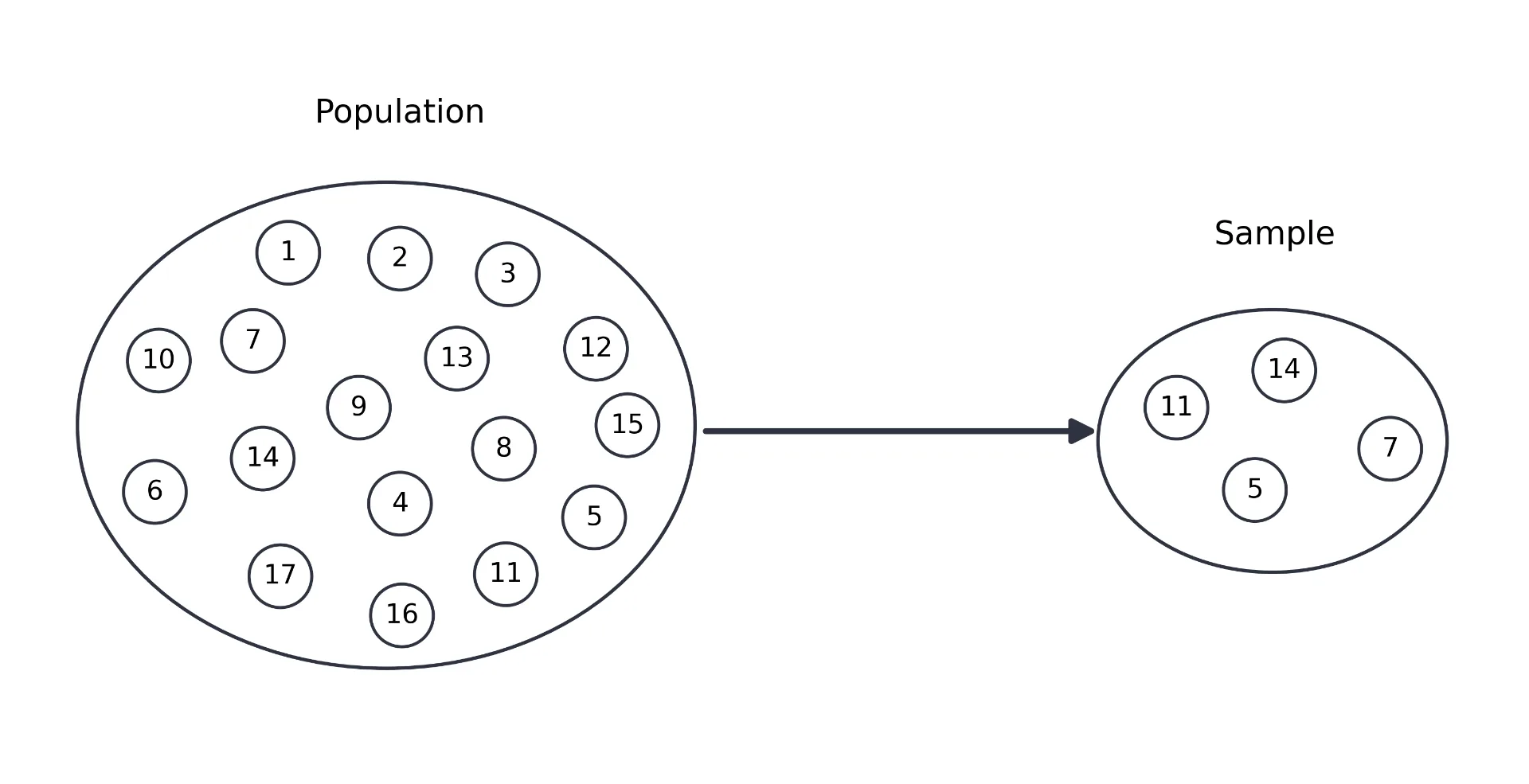
As shown above, a subset of a population is known as a sample.

When the data is too large to collect or compute, we often use sample data instead. But there is one important condition: the sample should be representative of the population and should not introduce systematic bias. This means that we should not select only a particular group of people in a way that could easily alter the outcome.

For example, if I only consider students who have scored 90% or above, the average marks will naturally be very high. But if we consider students with all kinds of marks, ranging from low to high, the sample is more likely to represent the actual population, and therefore, the results are more likely to be closer to the true population value.

The size of the population is denoted by N, while the size of the sample is denoted by n.

---

2. Why Divide by n − 1? Degrees of Freedom Explained

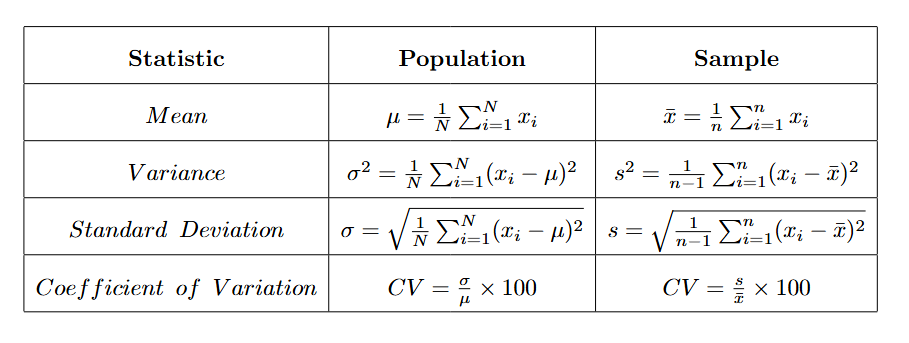
Here, a question may arise — why, in a sample, are we dividing by (n-1) and not by (n)?

To clear up this confusion, we need to learn something important.

Did you know that the sum of deviations from the mean is always 0?

Here is a small proof.

This is our sample mean:

x̄ = (x₁ + x₂ + ⋯ + xₙ) / n

If we multiply both sides by (n):

n·x̄ = x₁ + x₂ + ⋯ + xₙ

After expanding, we get the sum of the deviations of each sample point from the mean:

(x₁ − x̄) + (x₂ − x̄) + ⋯ + (xₙ − x̄) = 0

It will always be 0:

Σᵢ₌₁ⁿ (xᵢ − x̄) = 0

Now, let’s notice something. Suppose we have three deviations:

-2, 0, ?

Do we really need all three deviations? From the other two, we can easily say that the third one has to be (+2). That’s the only value that will make the sum equal to 0.

So, out of these 3 deviations, we can independently choose only 2. The last one is automatically determined by the other two.

Therefore, in general, if we have (n) deviations from the sample mean, only (n-1) of them can vary independently because their sum must be 0. This is where we get our first intuition for Degrees of Freedom.

There is one more important point. When we calculate sample variance, we are using the sample mean instead of the true population mean. Because of this, dividing by (n) would systematically make our estimate of variance a little too small. Dividing by (n-1) corrects this bias and gives us an unbiased estimate of the population variance.

Now you might be wondering: why did we take such a long route through populations, samples, and degrees of freedom before even talking about skewness? Because skewness and kurtosis are statistical measures, and to properly understand their formulas, we need to understand where population and sample formulas come from.

---

3. Moments: The Building Blocks of Shape

Before we move on to the main topic, there is one more important concept to cover: Moments.

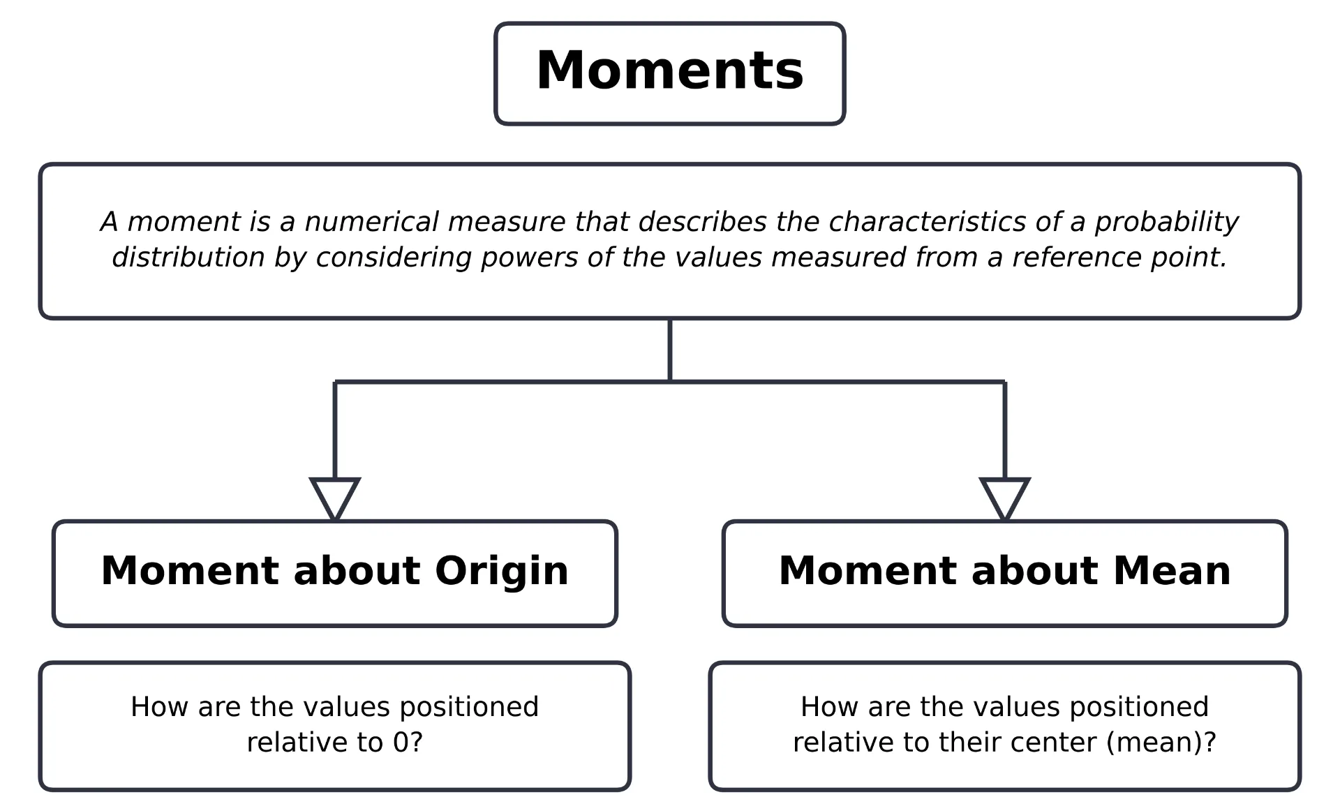
We have four central moments:

• First Central Moment → 0
• Second Central Moment → Variance
• Third Central Moment → Related to Skewness
• Fourth Central Moment → Related to Kurtosis

We have already covered Mean and Variance, which correspond to the first raw moment and second central moment, respectively. Here we take a deep dive into the Third and Fourth Central Moments and see how, after standardization, they lead to measures of Skewness and Kurtosis.

First Central Moment → 0:

μ₁ = E[(X − μ)]

Second Central Moment → Variance:

μ₂ = E[(X − μ)²]

Third Central Moment → Related to Skewness:

μ₃ = E[(X − μ)³]

Fourth Central Moment → Related to Kurtosis:

μ₄ = E[(X − μ)⁴]

These population moments are defined using the population distribution. If we want to calculate the corresponding sample moments, we replace the population expectation with the corresponding sample average:

mᵣ = (1/n) Σᵢ₌₁ⁿ (xᵢ − x̄)ʳ

---

4. Skewness: Measuring Asymmetry

4.1 Symmetric vs. Skewed Distributions

A distribution describes how the values of a variable are spread and how frequently different values or ranges of values occur. We can simply think of it as a map of our data.

This map could be Symmetric or Non-Symmetric.

A symmetric distribution looks like this:

Non-symmetric distributions are further classified into two types — right-skewed and left-skewed:

People often get confused because they consider the side with more of the distribution to be the side corresponding to its name. There is one key thing to remember: always look at the tail.

• If the long tail extends toward the right, it is Right-Skewed (Positively Skewed).
• If the long tail extends toward the left, it is Left-Skewed (Negatively Skewed).

4.2 Mean, Median and Mode in Skewed Data

It is also useful to observe how the Mean, Median, and Mode are positioned in these three distributions.

For a Left-Skewed (negatively skewed) distribution → Mean < Median < Mode.

For a symmetric normal distribution → Mean ≈ Median ≈ Mode.

For a Right-Skewed (positively skewed) distribution → Mean > Median > Mode.

The stretch in the tail of a skewed distribution pulls the mean in the direction of the tail, which is why the mean and median diverge as skewness increases.

4.3 From the Third Central Moment to Skewness

The third central moment captures asymmetry in a distribution. When deviations from the mean are cubed, positive and negative deviations no longer cancel symmetrically — large deviations on one side dominate, giving the moment a sign and magnitude that reflect the direction and degree of asymmetry.

The population third central moment is:

μ₃ = E[(X − μ)³]

To make this scale-independent, we divide by the cube of the standard deviation, yielding the population skewness:

γ₁ = μ₃ / σ³

4.4 Sample Skewness: Fisher–Pearson and Bias Correction

When working with sample data, the most widely used formula is the adjusted Fisher–Pearson standardized moment coefficient:

G₁ = [n / ((n−1)(n−2))] · Σᵢ₌₁ⁿ ((xᵢ − x̄) / s)³

where s is the sample standard deviation. The correction factor n / ((n−1)(n−2)) adjusts for the bias introduced by estimating the mean from the same sample. This is the formula used by default in software such as Microsoft Excel and many statistical packages.

4.5 How to Interpret Skewness Values

Skewness value	Interpretation
≈ 0	Approximately symmetric
> 0	Right-skewed (positive skew)
< 0	Left-skewed (negative skew)
|skewness| < 0.5	Fairly symmetric
0.5 ≤ |skewness| < 1	Moderately skewed
|skewness| ≥ 1	Highly skewed

---

5. Kurtosis: It’s About Tails, Not Peaks

5.1 What Kurtosis Really Measures

Kurtosis is commonly described as a measure of the “peakedness” of a distribution, but this framing is misleading. Kurtosis is more accurately understood as a measure of tail heaviness — specifically, how much of the distribution’s variance is driven by extreme values far from the mean.

A distribution with high kurtosis has heavier tails and more frequent outliers than a normal distribution. A distribution with low kurtosis has lighter tails and fewer extreme values.

5.2 Why the Fourth Power?

The fourth central moment uses the fourth power of deviations from the mean:

μ₄ = E[(X − μ)⁴]

Raising deviations to the fourth power amplifies large deviations dramatically while keeping the result non-negative. This makes the fourth moment especially sensitive to extreme values in the tails, which is precisely what kurtosis is designed to capture.

5.3 Excess Kurtosis: Where Does the “3” Come From?

The raw kurtosis of a normal distribution equals 3. To make interpretation easier, excess kurtosis subtracts 3 so that the normal distribution serves as a baseline of 0:

Excess Kurtosis = (μ₄ / σ⁴) − 3

This means:

• Excess kurtosis > 0 → heavier tails than normal
• Excess kurtosis = 0 → tails similar to normal
• Excess kurtosis < 0 → lighter tails than normal

Most software, including SciPy and pandas, reports excess kurtosis by default.

5.4 Leptokurtic, Mesokurtic and Platykurtic Distributions

Term	Excess kurtosis	Tail behavior
Leptokurtic	> 0	Heavy tails, more outliers
Mesokurtic	≈ 0	Normal-like tails
Platykurtic	< 0	Light tails, fewer outliers

A classic example of a leptokurtic distribution is the t-distribution, which has heavier tails than the normal distribution. The uniform distribution is platykurtic.

5.5 Sample Kurtosis and Fisher’s Correction

The bias-corrected sample excess kurtosis formula is:

G₂ = [(n(n+1)) / ((n−1)(n−2)(n−3))] · Σᵢ₌₁ⁿ ((xᵢ − x̄) / s)⁴ − [3(n−1)² / ((n−2)(n−3))]

This correction, known as Fisher’s correction, adjusts for the bias that arises when both the mean and variance are estimated from the same sample.

5.6 Skewness vs. Kurtosis: The Memory Map

Measure	Moment	What it captures
Skewness	3rd central moment	Direction and degree of asymmetry
Kurtosis	4th central moment	Tail heaviness and outlier tendency

---

6. Calculating Skewness and Kurtosis in Python

Python provides several straightforward ways to compute skewness and kurtosis. The scipy.stats module and pandas are the most common tools.

import numpy as np
import pandas as pd
from scipy import stats

# Generate sample data
np.random.seed(42)
data = np.random.exponential(scale=2, size=1000)

# Using scipy
skewness = stats.skew(data)
kurtosis = stats.kurtosis(data)  # excess kurtosis by default

print(f"Skewness: {skewness:.4f}")
print(f"Excess Kurtosis: {kurtosis:.4f}")

# Using pandas
series = pd.Series(data)
print(f"Pandas Skewness: {series.skew():.4f}")
print(f"Pandas Kurtosis: {series.kurt():.4f}")

Both scipy.stats.kurtosis and pandas.Series.kurt() return excess kurtosis (normal distribution baseline = 0) by default. To get the raw kurtosis from SciPy, pass fisher=False.

---

7. Taming Skewness: Data Transformations

Many machine learning algorithms assume that features are approximately normally distributed. When features are heavily skewed, applying a transformation can improve model performance and the validity of statistical tests.

7.1 Log Transformation

The log transformation is one of the most common remedies for right-skewed data:

x' = log(x)

It compresses large values and spreads out small values. It requires all values to be strictly positive (x > 0).

import numpy as np
data_log = np.log(data)

7.2 Square Root Transformation

A milder transformation than log, suitable for moderately right-skewed data:

x' = √x

Requires non-negative values (x ≥ 0).

data_sqrt = np.sqrt(data)

7.3 Cube Root Transformation

The cube root transformation can handle zero and negative values, making it more flexible:

x' = x^(1/3)

data_cbrt = np.cbrt(data)

7.4 Box-Cox Transformation

The Box-Cox transformation finds the optimal power parameter λ that makes the data most normal-like:

x'(λ) = (xˡ − 1) / λ,  if λ ≠ 0
x'(λ) = log(x),         if λ = 0

Requires strictly positive values.

from scipy import stats
data_boxcox, lambda_val = stats.boxcox(data)
print(f"Optimal lambda: {lambda_val:.4f}")

7.5 Yeo-Johnson Transformation

The Yeo-Johnson transformation is an extension of Box-Cox that supports zero and negative values:

from sklearn.preprocessing import PowerTransformer

pt = PowerTransformer(method='yeo-johnson')
data_yj = pt.fit_transform(data.reshape(-1, 1))

It is generally the safest default choice when the sign and range of values are unknown.

---

8. Standardization vs. Transformation

These two operations are often confused, but they serve different purposes.

Standardization

Standardization rescales data to have zero mean and unit variance (z-score normalization):

z = (x − x̄) / s

from sklearn.preprocessing import StandardScaler

scaler = StandardScaler()
data_scaled = scaler.fit_transform(data.reshape(-1, 1))

Key distinction: Standardization does not change the shape of a distribution. If the original data is right-skewed, the standardized data will still be right-skewed. Transformations (log, Box-Cox, Yeo-Johnson) change the shape; standardization only changes the scale and location.

In practice, transformation is applied first to address skewness, then standardization is applied to normalize the scale before feeding data into a model.

---

9. Kurtosis in Machine Learning

Kurtosis has several practical applications in machine learning workflows:

Outlier detection: High excess kurtosis signals heavy tails and a greater likelihood of extreme values. Features with high kurtosis warrant closer inspection before modeling, as outliers can distort distance-based algorithms (e.g., k-NN, k-means) and linear models.

Feature selection: Kurtosis can serve as a quick filter during EDA. Features with very high or very low kurtosis may require transformation or special handling.

Financial modeling: Many financial return distributions are leptokurtic — they exhibit more extreme events than a normal distribution would predict. Models that assume normality (e.g., some risk models) can underestimate tail risk when kurtosis is ignored.

Independent Component Analysis (ICA): ICA explicitly uses kurtosis (or related measures of non-Gaussianity) to separate mixed signals. The FastICA algorithm maximizes non-Gaussianity, often measured via kurtosis or negentropy, to find independent components.

Anomaly detection: Features with excess kurtosis significantly different from zero can indicate that a distribution is a mixture of subpopulations, which may be relevant for anomaly or fraud detection.

---

10. A Practical EDA Workflow

The following workflow integrates skewness and kurtosis checks into a standard exploratory data analysis process:

1. Compute descriptive statistics including mean, median, standard deviation, skewness, and kurtosis for each numerical feature.
2. Visualize distributions using histograms and KDE plots to confirm what the statistics suggest.
3. Flag highly skewed features (|skewness| ≥ 1) for transformation.
4. Flag high-kurtosis features (excess kurtosis > 3 or < −1) for outlier investigation.
5. Apply appropriate transformations (log, square root, Box-Cox, or Yeo-Johnson) based on the data range and skewness direction.
6. Recheck skewness and kurtosis after transformation to confirm improvement.
7. Apply standardization after transformation if the model requires it.

import pandas as pd
import numpy as np
from scipy import stats

def distribution_summary(df):
    results = []
    for col in df.select_dtypes(include=np.number).columns:
        results.append({
            'feature': col,
            'mean': df[col].mean(),
            'median': df[col].median(),
            'std': df[col].std(),
            'skewness': df[col].skew(),
            'excess_kurtosis': df[col].kurt()
        })
    return pd.DataFrame(results)

Running this function on a dataset before modeling gives a quick snapshot of which features need attention and what kind of preprocessing they require.

---

11. Supporting Materials

The Python code used to generate the distribution plots and statistical examples throughout this article is available as a companion notebook. The visualizations were created using Matplotlib and Seaborn, and the statistical computations use NumPy, SciPy, and pandas.

---

12. Resources

• SciPy stats documentation
• Pandas descriptive statistics
• Scikit-learn preprocessing: PowerTransformer
• Joanes, D. N., & Gill, C. A. (1998). Comparing measures of sample skewness and kurtosis. Journal of the Royal Statistical Society: Series D, 47(1), 183–189.
• DeCarlo, L. T. (1997). On the meaning and use of kurtosis. Psychological Methods, 2(3), 292–307.

Understanding skewness and kurtosis — and knowing how to act on them — is a foundational skill for anyone working with real-world data, where clean, normally distributed features are the exception rather than the rule.