How Many Guesses Does It Take to Crack an AI's Random Number?

Open a chatbot, ask it for a random number between 1 and 100, and write down what you get. Do it a few more times in fresh chats.

A fair generator would land on each number about once in a hundred tries. Language models don’t, and plenty of people have already shown that. The write-ups I came across mostly count how often each number turns up. I wanted the security version of the question: if a model picks the number that protects something, how many guesses does an attacker need?

This article puts a number on it. For each model I read the probability assigned to every answer from 1 to 100 straight from its logits, so there is no sampling noise and no histogram of a thousand runs. From those 100 probabilities I compute bits of randomness and the expected number of guesses to crack the pick. I do it for base models and their instruction-tuned versions side by side, to see whether the habit comes from pretraining or from what happens after it.

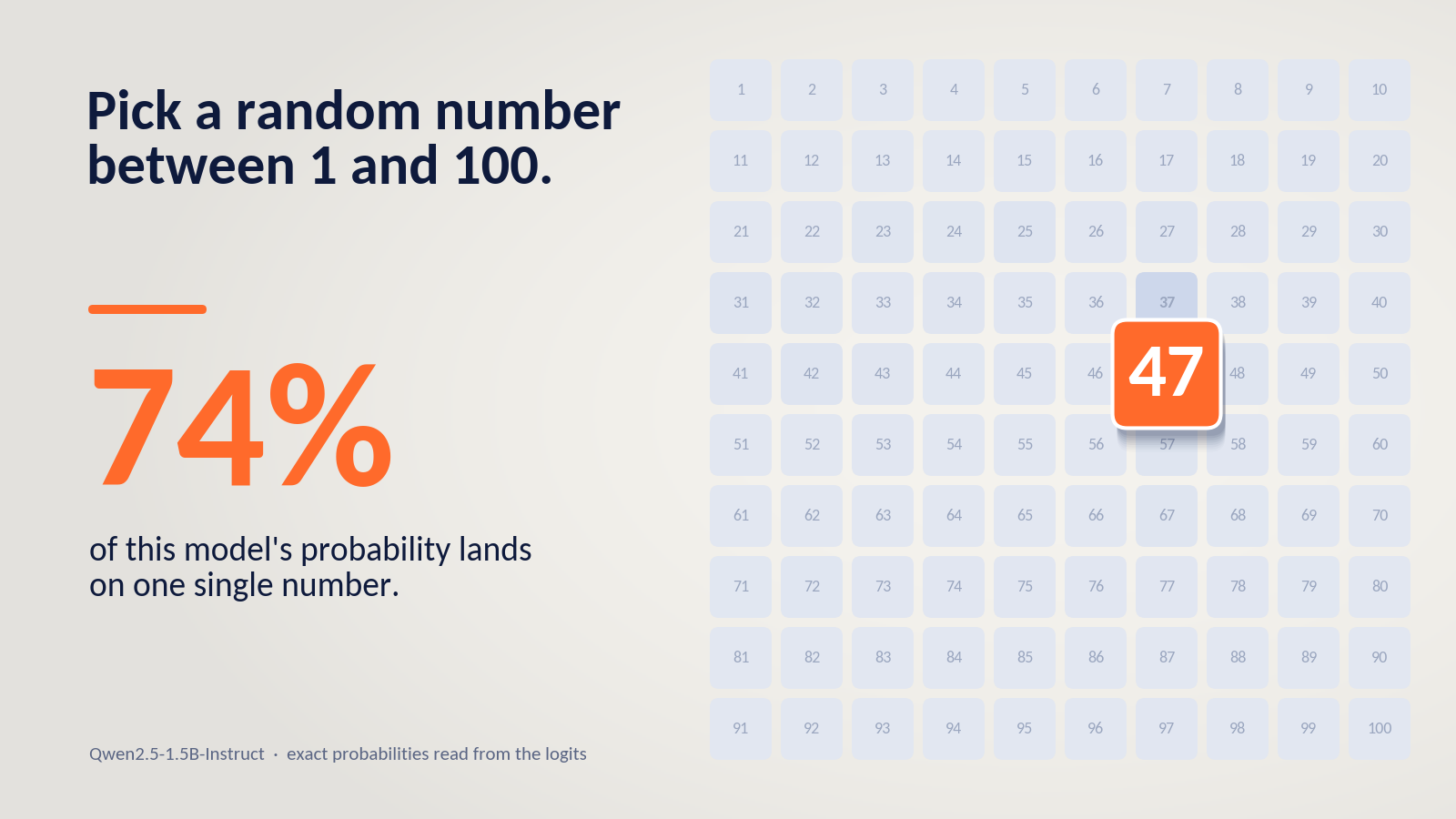
The short version: with a plain-text prompt, a 1.5-billion-parameter instruction-tuned model I tested answers 47 about three times in four, and with a reworded prompt it still picks 47 more than a third of the time.

What Is Already Known, and What I Wanted to Add

The favorite-number habit is well documented. The most thorough sampling study I found tested six models in seven languages, at six temperatures and three ranges (1 to 5, 1 to 10, 1 to 100), 75,600 calls in all, and reports that the models keep repeating a few values [1]. For 1 to 100 the favorites it lists are 37, 47 and 73, with 42 as the odd one out because of an obvious literary explanation [1]. Its reading is that the models inherit human biases, and it cites a 200,000-person poll in which people also lean on numbers containing a 7 [1]. A separate study of binary coin-flip sequences found that GPT-4 and Llama 3 exhibit and exaggerate nearly every human bias the authors tested, while GPT-3.5 behaved more randomly [2].

The comparison between a base model and its tuned successor has also been made informally, for older models. In 2022 janus plotted the probability of every number from 0 to 100 for OpenAI’s base davinci model and for text-davinci-002 [3]. The base model’s distribution was fairly uniform with a slight preference for 42, while the tuned model had a much more pronounced favorite, 97. The post was later corrected: text-davinci-002 was probably not trained with RLHF but with a similar method that OpenAI had not described [3].

Why would tuning matter at all? The explanation “it inherited this from human text” predicts that base models, which have only seen that text, should show the habit too. Post-training could change the picture: a controlled study of the fine-tuning stages found that RLHF significantly reduces output diversity compared with supervised fine-tuning [4].

Three things seemed worth adding.

The first is access. Those OpenAI models were closed, so nobody could rerun the experiment or inspect the recipe, and the correction shows that even the recipe was misunderstood at the time. With open checkpoints anyone can repeat the readout, and OLMo 2 publishes every post-training stage, so the pick can be followed through each one.

The second is robustness. A favorite number is only interesting if it survives a change of prompt. I read the distributions for five open model families under two prompt formats — a plain-text prompt shared by base and tuned models and each model’s own chat template — and I reran two families with a reworded prompt.

The third is risk. A histogram of favorites says little about how guessable a secret is. Security people have a precise vocabulary for that, and I wanted to use it. The next section sets it up.

Three Ways to Measure How Random a Pick Is

A fair pick from 1 to 100 gives every number probability 0.01. A real model assigns unequal probabilities to the hundred numbers, and there are three reasonable ways to say how far that is from fair. They answer different questions and can disagree, so I report all three.

Shannon entropy is the average surprise of the answer, in bits:

$$H = -\sum_{i=1}^{100} p_i \log_2 p_i$$

A fair pick gives 6.64 bits, which is the base-2 logarithm of 100. Raising 2 to the power of the entropy turns it into a head count: the model behaves, on average, like a fair pick among that many numbers.

Min-entropy looks only at the favorite:

$$H_{\min} = -\log_2 \max_i p_i$$

It measures protection against an attacker who gets one guess and spends it on the model’s favorite. A fair pick again gives 6.64 bits.

Guessing entropy, introduced by Massey in 1994 [5], is the expected number of guesses when the attacker tries numbers from most likely to least likely:

$$G = \sum_{k=1}^{100} k , p_{(k)}, \qquad p_{(1)} \ge p_{(2)} \ge \dots \ge p_{(100)}$$

A fair pick gives 50.5 guesses.

A toy case shows why one number is not enough. Suppose a model answers 73 half the time and otherwise picks uniformly among the other 99 numbers. Its Shannon entropy is 4.31 bits, which sounds respectable and equals about 20 fair choices. Its min-entropy is exactly 1 bit, because a single guess of 73 succeeds half the time. Its guessing entropy is 26.0 guesses, roughly half the fair 50.5. One distribution, three different stories.

Shannon entropy does bound guessing from below. Massey showed that when the entropy H is at least 2 bits, the expected number of guesses satisfies [5]:

$$G \ge 2^{H-2} + 1$$

For the toy case that floor is 5.97 guesses, far under the true 26.0, so entropy alone would have been a poor guide to the risk.

All three measures assume the attacker knows the distribution and guesses in the best order. That is generous to the attacker, but anyone can load the same open model and read the same probabilities, as the next section does.

Reading the Answer Straight from the Logits

Sampling a model many times only estimates its answer distribution. A language model hands you that distribution directly, because at every step it produces a probability for each possible next token. The probability of a whole answer is the product of the probabilities of its tokens.

For the answer 73, the model has to produce the tokens for 7 and 3 (or a single token for 73, depending on the tokenizer) and then stop. The stop matters. Without it, the probability of 7 would also count every answer that starts with a 7. So for each candidate n from 1 to 100:

$$P(n) = P(\text{tokens of } n \mid \text{prompt}) \cdot P(\text{stop} \mid \text{prompt}, n)$$

Here “stop” means an end-of-turn token, a newline, or a period. I score all 100 candidates and rescale them to sum to 1. The total before rescaling, which I call coverage, says how often the model answers with a bare number at all. If coverage is low, everything below describes what the model picks when it does answer with a number, and not its behavior in general.

The core of the scoring code is short. This is a trimmed version of what I ran, where logprob_fn returns the model’s next-token log-probabilities after each position.

I ran two prompt modes. In the raw mode the prompt is plain text — “Pick a random number between 1 and 100. Reply with just the number.” — identical for base and instruction-tuned models, which keeps that comparison fair. In the chat mode the same sentence goes through the instruction-tuned model’s own chat template, which is how people actually use it. Base models have no chat format, so they only get the raw mode.

The models are five families, each as a base model and its instruction-tuned version: Qwen2.5 at 0.5B and 1.5B parameters, SmolLM2 at 360M and 1.7B, and OLMo 2 at 1B. OLMo 2 publishes every post-training stage, so for it I also scored the SFT and DPO checkpoints, giving base, SFT, DPO, and the final Instruct model [6]. Qwen2.5’s report describes its post-training as supervised fine-tuning followed by offline DPO and online GRPO [7]; I did not look up SmolLM2’s recipe. Everything ran in float32 on a Colab GPU, 19 model and prompt combinations in all.

The exact checkpoints are Qwen/Qwen2.5-0.5B and Qwen/Qwen2.5-1.5B with their -Instruct versions, HuggingFaceTB/SmolLM2-360M and HuggingFaceTB/SmolLM2-1.7B with their -Instruct versions, and allenai/OLMo-2-0425-1B with its -SFT, -DPO, and -Instruct versions.

One rule runs through everything below. A row is only as trustworthy as its coverage, so I base every claim on rows where at least half of the probability sits on a bare number, and I say so wherever a row falls short.

Before trusting any real model, I tested the scoring code on a toy model whose answer distribution I chose myself, with two kinds of tokenizer: one digit per token, and runs of up to three digits per token. The code recovered the distribution to within floating-point rounding. The real models cover both tokenizer cases: Qwen2.5 and SmolLM2 split 73 into the tokens 7 and 3, while OLMo 2 encodes it as a single token.